Xgbda
Purpose
Gradient Boosted Tree Ensemble for classification (Discriminant Analysis) using XGBoost.
Synopsis
- model = xgbda(x,options); %identifies model using classes in x
- model = xgbda(x,y,options); %identifies model using y for classes
- pred = xgbda(x,model,options); %makes predictions with a new X-block
- valid = xgbda(x,y,model,options); %performs a "test" call with a new X-block with known y-classes
Please note that the recommended way to build and apply a Gradient Boosted Tree Ensemble for classification using XGBoost model from the command line is to use the Model Object. Please see this wiki page on building and applying models using the Model Object.
Description
XGB performs calibration and application of gradient boosted decision tree models for classification. These are non-linear models which predict the probability of a test sample belonging to each of the modeled classes, hence they predict the class of a test sample.
Note: In PLS_Toolbox version 9.5 and later the Python virtual environment must be configured in order to use this method. Find out more here: Python configuration.
Note: At this time, one cannot terminate Python methods from building by the conventional CTRL+C. For this reason you might want to save any important workspace variables before using this method.
Inputs
- x = X-block (predictor block) class "double" or "dataset".
- y = Y-block (predicted block) class "double" or "dataset". If omitted in a calibration call, the x-block must be a dataset object with classes in the first mode (samples). y can always be omitted in a prediction call (when a model is passed) If y is omitted in a prediction call, x will be checked for classes. If found, these classes will be assumed to be the ones corresponding to the model.
- model = previously generated model (when applying model to new data)
Outputs
- model = standard model structure containing the xgboost model (see Standard Model Structure). Feature scores are contained in model.detail.xgb.featurescores.
- pred = structure array with predictions
- valid = structure array with predictions
Options
options = a structure array with the following fields:
- display: [ 'off' | {'on'} ] governs level of display to command window.
- plots [ 'none' | {'final'} ] governs level of plotting.
- waitbar: [ off | {'on'} ] governs display of waitbar during optimization and predictions.
- preprocessing: {[] []}, two element cell array containing preprocessing structures (see PREPROCESS) defining preprocessing to use on the x- and y-blocks (first and second elements respectively)
- algorithm: [ 'xgboost' ] algorithm to use. xgboost is default and currently only option.
- classset : [ 1 ] indicates which class set in x to use when no y-block is provided.
- xgbtype : [ 'xgbr' | {'xgbc'} ] Type of XGB to apply. Default is 'xgbc' for classification, and 'xgbr' for regression.
- compression : [{'none'}| 'pca' | 'pls' ] type of data compression to perform on the x-block prior to calculaing or applying the XGB model. 'pca' uses a simple PCA model to compress the information. 'pls' uses either a pls or plsda model (depending on the xgbtype). Compression can make the XGB more stable and less prone to overfitting.
- compressncomp : [ 1 ] Number of latent variables (or principal components to include in the compression model.
- compressmd : [ 'no' |{'yes'}] Use Mahalnobis Distance corrected scores from compression model.
- compressmd : [ 'no' |{'yes'}] Use Mahalnobis Distance correctedscores from compression model.
- cvi : { { 'rnd' 5 } } Standard cross-validation cell (see crossval)defining a split method, number of splits, and number of iterations. This cross-validation is use both for parameter optimization and for error estimate on the final selected parameter values.Alternatively, can be a vector with the same number of elements as x has rows with integer values indicating CV subsets (see crossval).
- eta : Value(s) to use for XGBoost 'eta' parameter. Eta controls the learning rate of the gradient boosting.Values in range (0,1]. Using a single value specifies the value to use. Using a range of values specifies the parameters to search over to find the optimal value. Default is 3 values [0.1, 0.3, 0.5].
- max_depth : Value(s) to use for XGBoost 'max_depth' parameter. Specifies the maximum depth allowed for the decision trees. Using a single value specifies the value to use. Using a range of values specifies the parameters to search over to find the optimal value. Default is 6 values [1 2 3 4 5 6].
- num_round : Value(s) to use for XGBoost 'num_round' parameter. Specifies how many rounds of tree creation to perform. Using a single value specifies the value to use. Using a range of values specifies the parameters to search over to find the optimal value. Default is 3 values [100 300 500].
- strictthreshold : [0.5] Probability threshold for assigning a sample to a class. Affects model.classification.inclass.
- predictionrule : { {'mostprobable'} | 'strict' ] governs which classification prediction statistics appear first in the confusion matrix and confusion table summaries.
Algorithm
Xgbda is implemented using the XGBoost package. User-specified values are used for XGBoost parameters (see options above). See XGBoost Parameters for further details of these options.
The default XGBDA parameters eta, max_depth and num_round have value ranges rather than single values. This xgbda function uses a search over the grid of appropriate parameters using cross-validation to select the optimal XGBoost parameter values and builds an XGBDA model using those values. This is the recommended usage. The user can avoid this grid-search by passing in single values for these parameters, however.
Choosing the best XGBDA parameters
The recommended technique is to repeatedly test XGBDA using different parameter values and select the parameter combination which gives the best results. XGBDA searches over ranges of parameters eta, max_depth, and num_round, by default. The actual values tested can be specified by the user by setting the associated parameter option value. Each test builds an XGBDA model on the calibration data using cross-validation to produce a mis-classification rate result for that test. These tests are compared over all tested parameter combinations to find which combination gives the best cross-validation prediction (smallest mis-classification). The XGBDA model is then built using the optimal parameter setting.
XGBDA parameter search summary plot
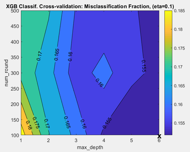
When XGBDA is run in the Analysis window it is possible to view the results of the XGBDA parameter search by clicking on the "Variance Captured" plot icon in the toolbar. If at least two XGB parameters were initialized with parameter ranges, for example eta and max_depth,, then a figure appears showing the performance of the model plotted against eta and max_depth (Fig. 1). The measure of performance used is the misclassification rate, defined as the number of incorrectly classified samples divided by the number of classified samples, based on the cross-validation (CV) predictions for the calibration data. The lowest value of misclassification rate is marked on the plot by an "X" and this indicates the values of the XGBDA eta and max_depth parameters which yield the best performing model. The actual XGBDA model is built using these parameter values. If all three parameters, eta, max_depth, and num_round have ranges of values then you can view the classification performance over the other variables' ranges by clicking on the blue horizontal arrow toolbar icon above the plot. In Analysis XGBDA the optimal parameters are also reported in the model summary window which is shown when you mouse-over the model icon, once the model is built. If you are using the command line XGBDA function to build a model then the optimal XGBDA parameters are shown in model.detail.xgb.cvscan.best.
This plot is useful to show you if you should consider changeing the range over which one or more parameters are tested over. If the best parameter set found, as denoted by the "X" mark occur at the edge of the searched range then it might be worthwhile extending the search range for that parameter to see if an even better parameter choice can be found in the extended domain.
- Fig. 1. Parameter search summary
Variable Importance Plot
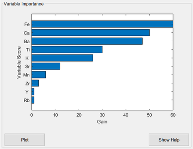
The ease of interpreting single decision trees is lost when a sequence of boosted trees is used, as in XGBoost. One commonly used diagnostic quantity for interpreting boosted trees is the "feature importance", or "variable importance" in PLS_Toolbox terminology. This is a measure of each variable's importance to the tree ensemble construction. It is calculated for each variable by summing up the “gain” on each node where that variable was used for splitting, over all trees in the sequence. "gain" refers to the reduction in the loss function being optimized. The important variables are shown in the XGBDA Analysis window when the model is built, ranked by their importance (Fig. 2).
- Fig. 2. Variable importance plot
XGBDA variable importance. 1) Right-click in the plot area to copy the indices of the important variables. Clicking on the "Plot" button opens a version of the plot which can be zoomed or panned. 2) Right-click also allows the choice of "Include only top N variables". This presents a new window where the value for N can be entered. This sets those top N variables as the Calibration X-block's included variables, and resets the model in the Analysis window to empty.
See Also
analysis, browse, knn, lda, lwr, pls, plsda, xgb, xgbengine, EVRIModel_Objects

