Calibration Transfer

About Calibration Transfer

Calibration transfer is useful when collecting data for similar samples on two or more different instruments (or on the same instrument at two or more different points in time). The goal is to create a model to compensate for differences in the instruments that can then be used to eliminate or reduce variation caused by the change in instrument. The following demonstration will show a simple example of creating a Piecewise Direct Standardization (PDS) model on some demonstration data included with PLS_Toolbox/Solo.

Available Model Types

• Direct Standardization
• Piecewise Direct Standardization
• Double Window Piecewise Direct Standardization

• Spectral Subspace Transformation
• Generalized Least-Squares Weighting
• Orthogonal Signal Correction
• Alignment of Matrices

Building Models (PDS Example)

Start the Interface

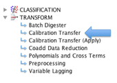
The easiest way to start the interface is by selecting Calibration Transfer within the Transform leaf in the browse interface:

Load Data

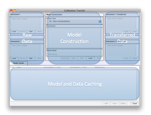
The general workflow in the GUI is from left to right. The first task when starting is to load raw data. This can be done with the Load button for Instrument 1 and 2. Go to the"dems" folder of PLS_Toolbox/Solo to find "nir_data.mat" and load 'spec1' and 'spec2' respectively. Once both datasets are loaded, you'll notice the Diff Bar located between the Instrument 1/2 panels gives an indication of how different the two datasets are:

Select Preprocessing

Next, select preprocessing for the data by clicking the Pre Pro button for Instrument 1 and add Mean Center. This data is quite "clean" so there's no need to consider more extensive preprocessing. Notice that after Preprocessing has been selected for Instrument 1 it is automatically added to Instrument 2. In general it is recommended that the same preprocessing be used for each instrument but Instrument 2 preprocessing can be changed by clicking on its Pre Pro button.

Construct Model

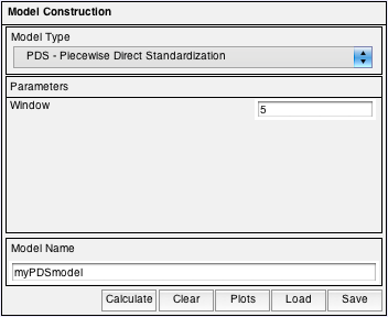
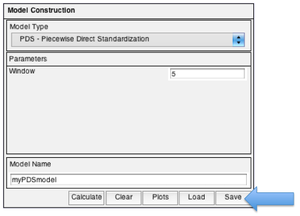
Now that the data is ready, it's time to set up the model. In the Model Construction area select Piecewise Direct Standardization (PDS) from the Model Type dropdown menu. Notice that the Window parameter appeared in the Parameters panel with a default value already entered along with a unique default Model Name. Either of these values can be changed by directly editing the value in the text box. For this demonstration we'll try a value of 5 for the Window and change the Model Name to "myPDSmodel".

The Plots button is also enabled and will open a dialog box allowing you to select any available plots to open in PlotGUI. At this point it's possible to plot the raw datasets and the data difference. Click Calculate to create the model.

Model Created

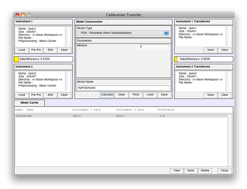
After a model has been calculated several things happen. The transferred data is added to its respective area, the model and all data (raw and transferred) are "cached" in the Model Cache panel, and additional plots are made available (via the Plots button).

From here you can explore the plots of your data and model, change parameters and create a new mode, or save your model and transferred data for further use. Clicking the View button will "reload" the selected cached model. Clicking the Save button will save the cached items (model, raw data, and transferred data) as a Matlab structure.

Applying Model to New Data (With the GUI)

From Calibration Transfer Window

1. Save the transfer model to the workspace. NOTE: that this is done with the save button in the Model Construction panel and not the Model Cache panel (see above).
2. Clear all of the current data and model, File>Clear>Clear All
3. Load the new data as Instrument 2.
4. Load the model you saved in step 1.
5. Click Calculate.

From Workspace

1. Save the transfer model to the workspace. NOTE: that this is done with the save button in the Model Construction panel and not the Model Cache panel (see above).
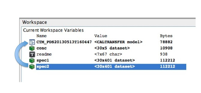
2. In the browse interface, drag and drop the data you wish to apply onto the model save in step 1.
3. A dialog box will open where you can name the transferred dataset.

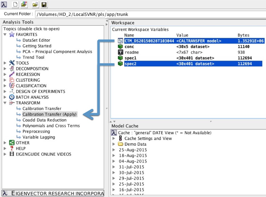
NOTE: The Calibration Transfer model and data can also be selected together and dropped on the "Calibration Transfer Apply" node. A dialog box will appear same as above asking to name the transferred dataset.

Applying Model to New Data (Command Line)

If you have a need to automate model application this can be done using the caltransfer function. The I/O looks similar to:

x2t = caltransfer(x2,transfermodel,options);

Where x2 is the Instrument 2 data and x2t is the Instrument 2 transferred data. Also see the caltransferdemo script for more examples.

Model-centric Calibration Transfer

If you have a model has been developed on a "master" instrument and is the basis of creating a "slave" model that includes a calibration transfer step in the preprocessing structure you may want to try Model-centric Calibration Transfer.