Advanced Preprocessing: Sample Normalization
Introduction
In many analytical methods, the variables measured for a given sample are subject to overall scaling or gain effects. That is, all (or maybe just a portion of) the variables measured for a given sample are increased or decreased from their true value by a multiplicative factor. Each sample can, in these situations, experience a different level of multiplicative scaling.
In spectroscopic applications, scaling differences arise from pathlength effects, scattering effects, source or detector variations, or other general instrumental sensitivity effects (see, for example, Martens and Næs, 1989). Similar effects can be seen in other measurement systems due to physical or chemical effects (e.g., decreased activity of a contrast reagent or physical positioning of a sample relative to a sensor). In these cases, it is often the relative value of variables which should be used when doing multivariate modeling rather than the absolute measured value. Essentially, one attempts to use an internal standard or other pseudo-constant reference value to correct for the scaling effects.
The sample normalization preprocessing methods attempt to correct for these kinds of effects by identifying some aspect of each sample which should be essentially constant from one sample to the next, and correcting the scaling of all variables based on this characteristic. The ability of a normalization method to correct for multiplicative effects depends on how well one can separate the scaling effects which are due to properties of interest (e.g., concentration) from the interfering systematic effects.
Normalization also helps give all samples an equal impact on the model. Without normalization, some samples may have such severe multiplicative scaling effects that they will not be significant contributors to the variance and, as a result, will not be considered important by many multivariate techniques.
When creating discriminant analysis models such as PLS-DA or SIMCA models, normalization is done if the relationship between variables, and not the absolute magnitude of the response, is the most important aspect of the data for identifying a species (e.g., the concentration of a chemical isn't important, just the fact that it is there in a detectable quantity). Use of normalization in these conditions should be considered after evaluating how the variables' response changes for the different classes of interest. Models with and without normalization should be compared.
Typically, normalization should be performed before any centering or scaling or other column-wise preprocessing steps and after baseline or offset removal (see above regarding these preprocessing methods). The presence of baseline or offsets can impede correction of multiplicative effects. The effect of normalization prior to background removal will, in these cases, not improve model results and may deteriorate model performance.
One exception to this guideline of preprocessing order is when the baseline or background is very consistent from sample to sample and, therefore, provides a very useful reference for normalization. This can sometimes be seen in near-infrared spectroscopy in the cases where the overall background shape is due to general solvent or matrix vibrations. In these cases, normalization before background subtraction may provide improved models. In any case, cross-validation results can be compared for models with the normalization and background removal steps in either order and the best selected.
A second exception is when normalization is used after a scaling step (such as autoscaling). This should be used when autoscaling emphasizes features which may be useful in normalization. This reversal of normalization and scaling is sometimes done in discriminant analysis applications.
Normalize
Simple normalization of each sample is a common approach to the multiplicative scaling problem. The Normalize preprocessing method calculates one of several different metrics using all the variables of each sample. Possibilities include:
| Name | Description | Equation* |
|---|---|---|
| 1-Norm |
Normalize to (divide each variable by) the sum of the absolute value of all variables for the given sample. Returns a vector with unit area (area = 1) "under the curve." |
|
| 2-Norm |
Normalize to the square root of the sum of the squared value of all variables for the given sample. Returns a vector of unit length (length = 1). A form of weighted normalization where larger values are weighted more heavily in the scaling. |
|
| Inf-Norm |
Normalize to the maximum value observed for all variables for the given sample. Returns a vector with unit maximum value. Weighted normalization where only the largest value is considered in the scaling. |
* Where, in each case, wi is the normalization weight for sample i, xi is the vector of observed values for the given sample, j is the variable number, and n is the total number of variables (columns of x).
The weight calculated for a given sample is then used to calculate the normalized sample, , using:
An example using the 1-norm on near infrared spectra is shown in the figure below. These spectra were measured as 20 replicates of 5 synthetic mixtures of gluten and starch (Martens, Nielsen, and Engelsen, 2003) In the original data (top plot), the five concentrations of gluten and starch are not discernable because of multiplicative and baseline effects among the 20 replicate measurements of each mixture. After normalization using a 1-norm (bottom plot), the five mixtures are clearly observed in groups of 20 replicate measurements each.
Figure: Effect of normalization on near-IR spectra of five synthetic gluten and starch mixtures. Original spectra (top plot) and spectra after 1-norm normalization (bottom plot) are shown.
From the Preprocessing window, the only setting associated with this method is the type of normalization (1-norm, 2-norm or inf-norm). There is currently no option to perform this normalization based on anything other than all selected variables.
From the command line, this method is performed using the normaliz function (note the unusual spelling of the function).
SNV (Standard Normal Variate)
Unlike the simple 1-Norm Normalize described above, the Standard Normal Variate (SNV) normalization method is a weighted normalization (i.e., not all points contribute to the normalization equally). SNV calculates the standard deviation of all the pooled variables for the given sample (see for example Barnes et al., 1989). The entire sample is then normalized by this value, thus giving the sample a unit standard deviation (s = 1). Note that this procedure also includes a zero-order detrend (subtraction of the individual mean value from each spectrum - see discussion of detrending, above), and also that this is different from mean centering (described later). The equations used by the algorithm are the mean and standard deviation equations:
where n is the number of variables, , is the value of the jth variable for the ith sample, and is a user-definable offset. The user-definable offset can be used to avoid over-normalizing samples which have near zero standard deviation. The default value for this offset is zero, indicating that samples will be normalized by their unweighted standard deviation. The selection of is dependent on the scale of the variables. A setting near the expected noise level (in the variables' units) is a good approximation.
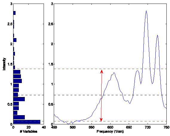
This normalization approach is weighted towards considering the values that deviate from the individual sample mean more heavily than values near the mean. Consider the example Raman spectrum in the figure below. The horizontal line at intensity 0.73 indicates the mean of the spectrum. The dashed lines at 1.38 and 0.08 indicate one standard deviation away from the mean. In general, the normalization weighting for this sample is driven by how far all the points deviate from the mean of 0.73. Considering the square term in the equation above and the histogram on the left of the figure, it is clear that the high intensity points will contribute greatly to this normalization.
Figure: Eample Raman spectrum (right plot) and corresponding intensity histogram (left plot). The mean of the spectrum is shown as a dashed line at intensity 0.73; one standard deviation above and below this mean are shown at intensities 1.38 and 0.08 and indicated by the arrow.
This approach is a very empirical normalization method in that one seldom expects that variables for a given sample should deviate about their mean in a normal distribution with unit variance (except in the case where the primary contribution to most of the variables is noise and the variables are all in the same units). When much of the signal in a sample is the same in all samples, this method can do very well. However, in cases where the overall signal changes significantly from sample to sample, problems may occur. In fact, it is quite possible that this normalization can lead to non-linear responses to what were otherwise linear responses. SNV should be carefully compared to other normalization methods for quantitative models.
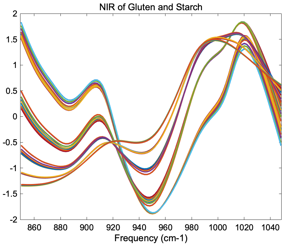
The figure below shows the result of SNV on the gluten and starch mixtures described earlier. Comparing the SNV results to the original spectra and 1-norm spectra shown in the "normalize" section above, it is obvious that SNV gives tighter groupings of the replicate measurements. In fact, SNV was originally developed for NIR data of this sort, and it behaves well with this kind of response.
Figure: Effect of SNV normalization on near-IR spectra measured of five synthetic gluten and starch mixtures.
From the Preprocessing window, the only setting associated with this method is the offset. There is currently no option to perform this normalization based on anything other than all selected variables. From the command line, this method is performed using the snv function.
MSC (Multiplicative Scatter Correction)
Multiplicative signal correction (MSC) is a relatively simple processing step that attempts to account for scaling effects and offset (baseline) effects (Martens and Næs, 1989). This correction is achieved by regressing a measured spectrum against a reference spectrum and then correcting the measured spectrum using the slope (and possibly intercept) of this fit. Specifically, MSC follows this procedure: Define x as a column vector corresponding to a spectrum to be standardized and r as a vector corresponding to the reference spectrum (often this is the mean spectrum of the calibration data set). The vectors are most often mean-centered according to:
where and are the mean centered vectors, and are the respective means, and is a vector of ones. The unknown multiplicative factor b is determined using:
and the corrected spectrum is then given by:
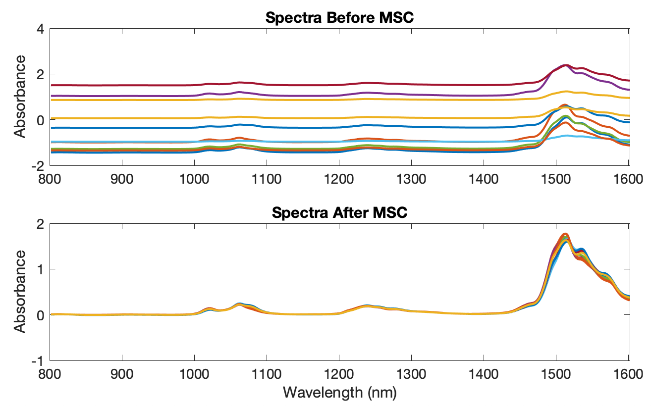
The figure below shows an example of MSC using NIR spectra of synthetic gasoline samples with added baseline and scaling effects. The spectra with artificial baseline and scaling effects are shown in the top plot. The corrected spectra are shown in the bottom plot. The corrected spectra were brought to within 0.03 absorbance units of the original spectra (not shown).
Figure: Example of Multiplicative Scatter Correction of artificial baseline and scaling effects.
The simulated baseline addition and subsequent correction can be done using the following commands:
» bspec = spec1.data(21:30,:);
» for i = 1:10, bspec(i,:) = bspec(i,:)*rand(1) + randn(1); end
» [sx,alpha,beta] = mscorr(bspec,mean(spec1.data(1:20,:)));
The first line creates a matrix of ten spectra. The second multiplies them by a random number between 0 and 1 and adds a random offset. The function mscorr is then used to correct the spectra using the mean of the first twenty spectra as the reference. The outputs of mscorr are the corrected spectra (sx), and the intercepts (alpha), and slope (beta) for the fit of each spectrum to the reference.
From the Preprocessing window, there are two settings which can be modified: intercept and spectral mode. The intercept option controls whether or not the intercept (i.e., in the last equation above) is used. The spectral mode setting defaults to 2 and can only be modified when x is a multiway matrix. This setting defines the data mode which is associated with the spectral dimension (i.e., the mode which should be used in the regression). There is currently no option to perform this normalization based on anything other than all selected variables.
From the command line, this method is performed using the mscorr function. The extended multiplicative scatter correction (EMSC) algorithm is a patented algorithm which can be purchased separately. The algorithm and use are described in the emscorr documentation pages.


