Umap
Purpose
Perform Unsupervised Uniform Manifold Approximation and Projection
Synopsis
- model = umap(x,options); %identifies model (calibration step)
- pred = umap(x,model); %applies model to new data (validation step)
- umap %Launches Analysis window with UMAP selected
Please note that the recommended way to build and apply a UMAP model from the command line is to use the Model Object. Please see this wiki page on building and applying models using the Model Object.
Description
UMAP is one of many tools to visualize high-dimensional data. Our software uses the Python (umap-learn package) implementation of the UMAP method. Their documentation can be found here: https://umap-learn.readthedocs.io/en/latest/. UMAP will model the input data as a "fuzzy" topological structure. The embeddings will come from a lower dimensional space that most closely resembles the topological structure of the original space. The embeddings will return n_component embeddings. E.g. for an M by N matrix, if the dimension of the embedded space (n_component) is K the embeddings will be of shape M by K.
Note: The PLS_Toolbox Python virtual environment must be configured in order to use this method. Find out more here: Python configuration. At this time, one cannot terminate Python methods from building by the conventional CTRL+C. Please take this into account and mind the workspace when using this method. This implementation ONLY performs Unsupervised Learning. Supervised UMAP Learning will be released at a later time.
Inputs
- x = X-block (2-way array class "double" or "dataset").
Optional Inputs
- model = existing UMAP model, onto which new data x is to be applied.
- options = discussed below.
Outputs
The output of UMAP is a model structure with the following fields (see Standard Model Structure for additional information):
- modeltype: 'UMAP',
- datasource: structure array with information about input data,
- date: date of creation,
- time: time of creation,
- info: additional model information,
- description: cell array with text description of model, and
- detail: sub-structure with additional model details and results.
Note: The embeddings of the UMAP model can be found under detail.umap.embeddings.
Options
options = a structure array with the following fields:
- display: [ 'off' | {'on'} ], governs level of display to command window,
- plots: [ 'none' | {'final'} ], governs level of plotting.
- warnings : [{'off'} | 'on'], Silence or display any potential Python warnings. Only visible in the MATLAB command window.
- preprocessing: {[]}, cell array containing a preprocessing structure (see PREPROCESS) defining preprocessing to use on the data (discussed below),
- n_neighbors: [ {'15'} ], Number of neighbors to consider. Controls the balance between local and global structure in the data.
- min_dist: [ {'0.1'} ], Minimum distance from data points in the low dimensional representation. Low values result in more clustered/clumped embeddings while a larger value results in a more even dispersal of points. This parameter should be set relative to the spread parameter.
- spread: [ {'1'} ], The effective scale of embedded points. In combination with min_dist this determines how clustered/clumped the embedded points are. This parameter should be set relative to the min_dist parameter.
- n_components: [ {'2'} ], The dimensionality of the reduced space.
- metric: [ {'euclidean'} | 'manhattan' | 'cosine' | 'mahalanobis' ], The metric used to calculate distance between data samples.
- random_state: [ {'1'} ], Random seed number. Set this to a number for reproducibility.
- blockdetails : [ {'standard'} | 'all' ], Extent of predictions and raw residuals included in model. 'standard' = none, 'all' x-block.
- compression: [ {'none'} | 'pca' ], Type of data compression to perform on the x-block prior to calculating or applying the UMAP model. 'pca' uses a simple PCA model to compress the information.
- compressncomp: [ {'2'} ], Number of latent variables (or principal components to include in the compression model).
- compressmd: [ {'yes'} | 'no' ], Use Mahalnobis Distance corrected.
The default options can be retrieved using: options = umap('options');.
PREPROCESSING
The preprocessing field can be empty [] (indicating that no preprocessing of the data should be used), or it can contain a preprocessing structure output from the PREPROCESS function. For example options.preprocessing = {preprocess('default', 'autoscale')}. This information is echoed in the output model in the model.detail.preprocessing field.
Connectivity Graph
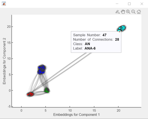
Starting with PLS_Toolbox/Solo 9.1, we have added the ability to generate a UMAP connectivity graph of UMAP embeddings. Since a UMAP model can be described as topological structure, we can represent this structure as a weighted graph. This plot is to be used to better understand the embeddings of a UMAP model and the relationships between the different embeddings. One can access the plot by clicking on the flask circle button ![]() in the toolbar in the UMAP interface. Below is an example of a UMAP connectivity graph with the ability to view each point and note the sample, class and label (if provided in the dataset object), and the number of connections it has with other embeddings. This example was generated using the arch demo dataset.
in the toolbar in the UMAP interface. Below is an example of a UMAP connectivity graph with the ability to view each point and note the sample, class and label (if provided in the dataset object), and the number of connections it has with other embeddings. This example was generated using the arch demo dataset.
Further reading on UMAP connectivity plots:
- https://arxiv.org/abs/2108.05525
- https://umap-learn.readthedocs.io/en/0.5dev/plotting.html#plotting-connectivity
Notes:
- Only applicable for UMAP models built with 2 or 3 components
- This plot can be slow to generate due the amount lines that must be drawn in the plot. This process can be sped up by decreasing the number of neighbors in the model
