Tools: Permutation Test
Permutation Test Tool
Some regression and preprocessing methods are so exceptionally good at finding correlation between the measured data (X- and Y-blocks) that the model becomes too specific and will only apply to that exact data. Such over-fit models are often useless for predictive applications or even exploratory interpretation purposes. In many cases, careful use of cross-validation and/or separate validation data will help identify when this has happened. Permutation tests are another way to help identify an overfit model as well as provide a probability that the given model is significantly different from one built under the same conditions but on random data. If the modeling conditions are over-fitting, they will often provide a fit to random data which is better than would be expected. Permutation tests use this condition to test for over-fitting.
Permutation tests involve repeatedly and randomly reordering the y-block, rebuilding the model with the current modeling settings after each reordering. For a regression problem, this means each sample is assigned a nominally "incorrect" y-value (although the distribution of y-values is maintained because every sample's y-value is simply re-assigned to a different sample.) In the case of classification models, reordering the y-block is equivalent to shuffling the class assignments on each sample, assigning samples to the "wrong" classes.
Such permutation examines the extent the modeling conditions might be finding "chance correlation" between the x-block and the y-block or over-filtering the data. After each permutation of the y-block, the predictions for each sample from cross-validation and self-prediction, and the RMSEC and RMSECV (see Using Cross-Validation) are recorded. The shuffling is repeated multiple times and several statistics are calculated for each permutation. The result is reported in two forms:
- A table of "Probability of Model Insignificance"
- A plot of Sum Squared Y (SSQY) versus Y-block correlation
When the tests are performed, the user is prompted for the number of iterations to use. The statistics being calculated for the table results are designed to operate with very few iterations (as few as one, in fact) but additional iterations help to confirm the results. Iterations are more critical for the SSQ Y plot. If the plot is not of interest, the number of iterations can be greatly reduced (down to 5 or 10, for example). Otherwise, iterations of 50, 100, 200 or more should be used.
See Permutetest for information on the command line function.
Probability Table
The probability table shows the probabilities (calculated using several different methods) that the predictions for the original, unperturbed model could have come from random chance. Put another way: these are the probabilities that the original model is not significantly different from one created from randomly shuffling the y-block. Results from three tests are shown:
- Wilcoxon - Pairwise Wilcoxon signed rank test
- Sign Test - Pairwise signed rank test
- Rand t-test - Randomization t-test
The result is reported as a probability that the models are not distinguishable at the given probability level. Thus a value of 0.05 indicates that the models are indistinguishable at the 5% limit, which is equivalent to saying they are significantly different at the 95% limit.
The tests utilize the prediction residuals:
where y is the perturbed y-values and is the model-estimated values for y. The comparison is between residuals obtained with an un-permuted y-block to those obtained with the permuted y-block.
In most publications, the tests are performed on the self-prediction residuals (those obtained when the model is built from all data and applied to the same data), but the permutation tests used here also include results for the cross-validated residuals (obtained when the model is built from a subset of data and applied to the left-out data.) The sensitivity of these two sources of residuals to overfitting depends on the noise sources and modeling conditions. The cross-validated residuals may be slightly more sensitive to detecting over-fitting because both permuted and un-permuted residuals will begin to grow significantly as the data are over-fit.
An example below shows an example in which the original model is very unlikely to be random.
Probability of Model Insignificance vs. Permuted Samples
For model with 1 component(s)

Y-column:  1
                     Wilcoxon     Sign Test     Rand t-test
Self-Pred (RMSEC) :   0.000        0.000          0.005
Cross-Val (RMSECV):   0.000        0.000          0.005
Compare this to the result obtained when the number of samples is decreased to 1/3 and the number of latent variables raised to 2. The all three tests on self-predictions are now indicating that the un-permuted model is probably not significantly different (at the 95% confidence level) from ones created with randomly permuted samples. Both the Sign and Randomization t-tests indicate the permuted and un-permuted models are similar for cross-validated residuals.
Probability of Model Insignificance vs. Permuted Samples
For model with 2 component(s)

Y-column:  1
                     Wilcoxon     Sign Test     Rand t-test
Self-Pred (RMSEC) :   0.085        0.186          0.076
Cross-Val (RMSECV):   0.021        0.060          0.099
For more details on the statistics shown in these tests, see the following publications:
- Edward V. Thomas, "Non-parametric statistical methods for multivariate calibration model selection and comparison", J. Chemometrics 2003; 17: 653–659.
- Hilko van der Voet "Comparing the predictive accuracy of models using a simple randomization test", Chemometrics and Intelligent Laboratory Systems 25 (1994) 313-323.
SSQ Y Plot
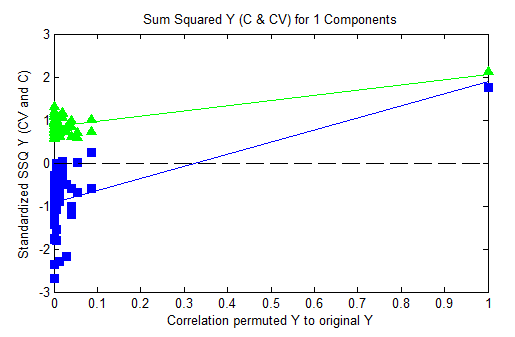
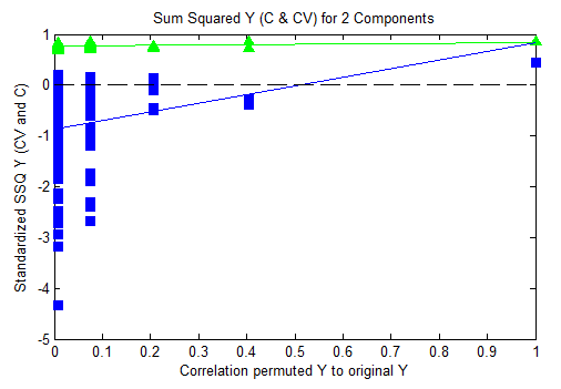
The SSQ_Y Plot shows fractional y-variance captured for self-prediction (calibration) and cross-validation versus the correlation of the permuted y-block to the original y-block.
For each permuted y-block, the root mean squared error of calibration and cross-validation (RMSEC and RMSECV, respectively) are calculated and stored. From these values, the fractional sum squared Y captured (SSQ Y) for the calibration (self-predictions) can be calculated from:
SSQY,C = 1-(SSEY,C/SSQY,Total)
Where SSEY,C is the sum squared error in Y self-prediction, SSQY,Total is the total sum squared Y response) and for cross-validated predictions from:
SSQY,CV = 1-(SSEY,CV/SSQY,Total)
The SSQ_Y,C is expected to increase up to a value of "1" when the model is capturing all the y-block response. The SSQ_Y,CV is expected to be about the same as the SSQ_Y,C as long as the model is not over-fit.
The SSQY,C and SSQY,CV are shown in centered and standardized form, meaning the y-axis value of any model's result indicates how far away from the data mean that point is in standard deviations. In general, the cross-validated and self-prediction values should be relatively close to each other, but should be significantly less than the results for the non-permuted y-block (on the far right side of the plot.) The further away the un-permuted results are from the mean, the more unlikely it is the original model is over-fit. The y-value of the un-permuted model SSQ results indicates the nth standard deviation at which the original model can be considered to fall. The higher the y-value, the more likely it is that the original model is significant and not over-fit.
An example (corresponding to the examples given above) of a good permutation result where the unpermuted results are several standard deviations away from the bulk of the corresponding permuted results:
And the same data with 1/3 the number of samples and 2 latent variables. These results indicate a likely overfit of the model:


