Constructing Image DataSets: Difference between revisions
imported>Scott |
imported>Scott |
||
| Line 42: | Line 42: | ||
we’re loading the JPEG from above directly into the Analysis GUI (start the Analysis | we’re loading the JPEG from above directly into the Analysis GUI (start the Analysis | ||
GUI from the command line by using the command analysis). | GUI from the command line by using the command analysis). | ||
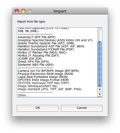
[[Image:Importmenu.jpg|Import Data List Box]] | [[Image:Importmenu.jpg|Import Data List Box]] | ||
After you've selected the file you wish to import, you're prompted by the imageload GUI | After you've selected the file you wish to import, you're prompted by the imageload GUI | ||
to specify what modes are spatial and which mode you'd like them unfolded to. | to specify what modes are spatial and which mode you'd like them unfolded to. | ||
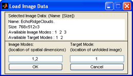
[[Image:ImageLoadGUI.png|Image Load GUI ]] | [[Image:ImageLoadGUI.png|Image Load GUI ]] | ||
Since the spatial data resides in the first two modes (768x512 pixels) we enter "1,2" in | Since the spatial data resides in the first two modes (768x512 pixels) we enter "1,2" in | ||
Revision as of 15:29, 14 November 2008
Building image DSOs can be accomplished via a gui or from the command line. Using buildimage you can designate the folded image data, the spatial modes (dimensions) of the image, the target mode where image is unfolded to, and a name for the DSO. Alternatively you can run imageload and designate this information via a GUI. Imageload is also called from the Analysis and Dataset Editor applications via File/Import menu.
From the Command Line
The following example uses the EchoRidgeClouds.jpeg image from the MIA_Toolbox/dems folder. This JPEG image contains RGB (Truecolor) information of size N x M x 3 where N and M are the pixel (spatial) dimensions. The following commands will load the image using the Matlab image read command imread then unfold the image into the first mode of an image dataset.
>> myimage = imread('EchoRidgeClouds.jpeg');
>> myimage = buildimage(myimage ,[1 2], 1, 'myNewImage')
myimage =
       name: myNewImage
       type: image
     author:
       date: 03-Oct-2005 10:31:03
    moddate: 03-Oct-2005 10:31:03
       data: 393216x3 [double]
  imagesize: 768x512
  imagemode: 1
      label: {2x1} [array (char)]
               Mode 1  [: ]
               Mode 2  [: ]
axisscale: {2x1} [vector (real)]
...
What if you have an existing DSO with image data in it? Use the exact same command:
>> myimage = buildimage(mydso ,[1 2], 1, 'myNewImage')
The last input to buildimage, 'myNewImage', renames the dataset (the default name is the variable name). The default setting for buildimage is to handle 3 dimensional data (three modes), see the documentation for specific settings.
From a GUI
In PLS_Toolbox GUIs, loading images is easy. You'll notice extra selections in the Import menu for images: File/Import Data/X Block. In this example we’re loading the JPEG from above directly into the Analysis GUI (start the Analysis GUI from the command line by using the command analysis).
After you've selected the file you wish to import, you're prompted by the imageload GUI
to specify what modes are spatial and which mode you'd like them unfolded to.
Since the spatial data resides in the first two modes (768x512 pixels) we enter "1,2" in
the Image Modes text box. Generally you put unfolded data into mode 1 of the new
image dataset, so we'll use the default value of "1" in the Target Mode text box. Clicking
OK loads the data into Analysis.
If you build a PCA model on this data you'll notice two things, an extra button on the
toolbar and different behavior when viewing data or scores.
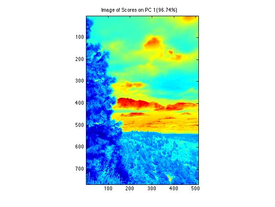
The extra button opens the imagegui tool, see the PLS_Toolbox documentation for more information how imagegui works or type help imagegui at the command line. Also note that imagegui needs at least 2 pc's calculated to be enabled. Viewing data and scores will display information in its "folded", image form. In this example the 2 pc model scores plot displays in the original image spatial dimensions.
Most methods in the analysis GUI are image “enabled” in that they will automatically work on image data (parafac will still operate on images but won't display "folded" image data). Be aware of size involved in image data. Large volumes of data will require extended amounts of time and computer memory to analyze.


