Getting Started With Matlab

About MATLAB

MATLAB, an acronym for MATrix LABoratory, is a product of The MathWorks, Inc., (Natick, MA). MATLAB is built around the LAPACK and BLAS linear algebra engines. It is a programming/computational environment especially suited to problems in matrix algebra, allowing the user to do matrix computations in a computing language that looks very much like standard linear algebra notation. MATLAB, which is required to run PLS_Toolbox, is not an inexpensive package (as you probably already know). However, because of its large collection of built-in functions, powerful graphics, easy-to-learn language, extensibility, and flexible environment, it is a great value. Another positive aspect of MATLAB is that it is available for many platforms, including Mac OS X, Microsoft Windows, Unix, and Linux. Thus, PLS_Toolbox can be run on all these platforms.

MATLAB can be used in the "command line" mode, where single line commands are entered at the command prompt (>>), executed immediately, and the results displayed. MATLAB contains hundreds of commands; a complete description of MATLAB commands is contained in the manuals provided with the software and through onscreen help.

We have continued to expand our use of GUIs (Graphical User Interfaces) with PLS_Toolbox and Solo. All of our major chemometric routines are available via GUIs and include a sophisticated layout allowing quick access to tools and information, including contextual menus, short cuts, and integrated help.

Before entering the PLS_Toolbox GUI environment the user must first enter and navigate the command mode. Thus, some minimal understanding of the command mode is required even of the beginner. Although a good number of powerful methods are available through our GUIs, there are still several routines only accessible from the command line. It is the intention of this section to get the new MATLAB user sufficiently comfortable with the command line mode to load data, do simple manipulations of data, execute PLS_Toolbox GUI routines, and finally save data and models to permanent media.

Startup

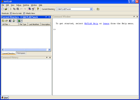
After starting MATLAB the MATLAB Desktop will appear, the default three-part window look similar to the figure below. The Desktop is also known as an Integrated Development Environment (IDE). In older version of Matlab (pre 2012b), clicking the Start button in the lower left-hand corner will display a list of MATLAB tools, shortcuts, and documentation. Mousing over the top item, MATLAB, will display a submenu that should have PLS_Toolbox listed at or near the bottom. Should it not be found, please install PLS_Toolbox as described here.

Default MATLAB desktop at startup.

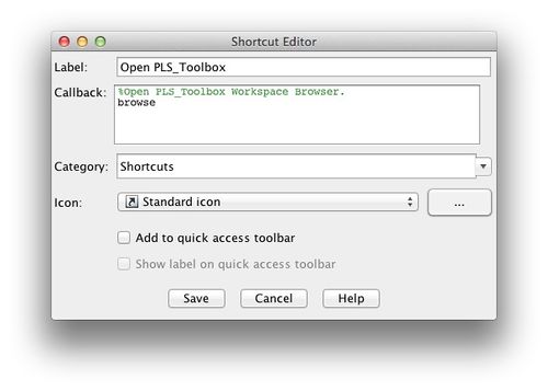
In new versions of MATLAB (2012b and newer), create a shortcut to start PLS_Toolbox.

Command Window

The heart of MATLAB is the Command Window. It is where commands can be directly entered by typing them followed by a return. The >> prompt shows that the Command Window is ready for entering a command. Together, MATLAB and PLS_Toolbox contain hundreds of commands in the form of scripts and functions. A script is simply a series of commands that are executed, as if they were individually typed in at the >> prompt, when the command is called. A function is similar to a script except that arguments are passed to it when it is called and it returns other arguments calculated by the function. A script runs in the base Workspace and does not return value. Once a script or function has been defined, it can be called from the command window or by other functions or scripts.

Terminology Note

"Command Window" and "Command Line" are used interchangeably throughout this documentation. When asked to enter a command "at the Command Line" or "in the Command Window" is simply means to type the command at the prompt >>.

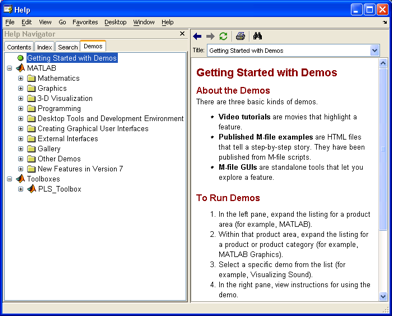
One of the most useful commands for a beginner is demo. (Note that MATLAB is case sensitive and the commands Demo, DEMO and demO would be interpreted by MATLAB as different (and most likely undefined) commands.) If the user types demo in the Command Window (followed by a return), the MATLAB help browser will appear at the Getting Started with Demos page. It is well worth the time for a new user to explore both MATLAB and PLS_Toolbox demonstrations.

Another useful command is the help command. It is executed by typing help followed by the name of the command. For example, type help demo to see instructions on using the demo command. The demo command requires that you remember the exact name of the command. If you cannot remember the command name, then use the lookfor command followed by a key word. For example, lookfor demonstration will cause MATLAB to search for all commands that use the word demonstration in the first line of their help file.

MATLAB Help demos window.

Finally, provided the Documentation files have been loaded into the computer when MATLAB was installed, detailed help may be obtained using the Help menu choice in the top MATLAB command bar. A record of executed commands can be viewed by scrolling up the Command Window or by examining the Command History window.

For more information about Matlab and using the Desktop try The MathWorks website.

Entering Data at the Command Window

Before MATLAB can do calculations, it needs data to work on. Typing the following command:

>> A = [2 5 3 6
7 3 2 1
5 2 0 3]

defines the variable A equal to the matrix enclosed within the square brackets. The spaces between the numbers delineate the columns and each return starts a new row. The same results are obtained if we use the command:

>> A = [2 5 3 6; 7 3 2 1; 5 2 0 3]

where the returns have been replaced by semicolons. Either way MATLAB will respond by typing the resulting matrix:

A =

   2   5   3   6
   7   3   2   1
   5   2   0   3

If you do not wish to see MATLAB echo (print out) the result, end the command with a semicolon. For example, if you type:

>> A = [2 5 3 6; 7 3 2 1; 5 2 0 3];

the variable A will be defined as before, but MATLAB will not echo the result. When working with very large matrices, the use of the semicolon can prevent thousands of elements from being printed on the screen.

Importing Data with Matlab

Typing in data by hand can become very tedious for large data sets. MATLAB can read a variety of files from other major programs that store data. For example, we may wish to load an Excel file (included as demonstration data with PLS_Toolbox and shown below) containing data for six brands of beer and eleven properties for each beer (Analytical data courtesy The Gambrinus Company, San Antonio, TX).

	Specific Gravity	App Extr	Alcohol (%w/w)	Real Ext	O.G.	RDF	Calories	pH	Color	IBU	VDK (ppm)
Shea's Irish	1.01016	2.60	3.64	4.29	11.37	63.70	150.10	4.01	19.0	16.1	0.02
Iron Range	1.01041	2.66	3.81	4.42	11.82	64.00	156.30	4.33	11.6	21.1	0.04
Bob's 1st Ale	1.01768	4.50	3.17	5.89	12.04	52.70	162.70	3.93	30.7	21.1	0.11
Manns Original	1.00997	2.55	2.11	3.58	7.77	54.90	102.20	4.05	58.9	18.2	0.05
Killarney's Red	1.01915	4.87	3.83	6.64	14.0	54.30	190.20	4.36	12.3	17.9	0.02
Killian's Irish	1.01071	2.74	3.88	4.48	12.0	64.10	158.80	4.28	53.0	14.2	0.03

These data can be found in the file Redbeerdata.xls in the PLS_Toolbox/dems directory.

Note

PLS_Toolbox includes several functions for reading .xls and other data files directly into the DataSet Object format typically used with its functions (see, for example, xlsreadr). However, here we will use only the built-in MATLAB-based functions in order to more fully explore MATLAB commands.

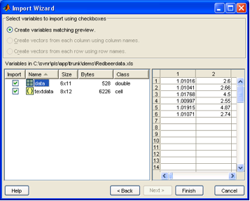
Redbeerdata.xls may be loaded into MATLAB by first selecting the File/Import Data... menu from the Command Window. Once the appropriate file has been found and chosen in the Import window, the data Import Wizard will present the window shown below.

Matlab Import Wizard with Redbeerdata.xls.

The Import Wizard has divided the data into a numerical data matrix (data) and a text data matrix (textdata). Notice that the matrix data is a 6 x 11 matrix of numbers in this case. (Matrix notation always refers to rows first followed by the columns.) The variable textdata is an 8 x 12 matrix of text cells. Highlight the variable data and one can examine the first 10 x 10 part of the matrix to make sure that MATLAB has properly delineated the numerical data. Highlighting the variable textdata allows the user to see that it is made of text cells from the column and row labels, and that the numerical data have been removed, leaving blank cells.

Clicking on the Finish button will complete the loading of the data into MATLAB.

Examining the MATLAB Workspace

We can examine MATLAB’s data memory or Workspace by typing whos at the prompt.

>> whos

 Name        Size     Bytes  Class

 data        6x11       528  double array
 textdata    8x12      6226  cell array

Grand total is 395 elements using 6226 bytes

If you prefer, the Workspace can be examined by choosing Workspace in the View menu. A Workspace window will appear.

When we examine the Workspace after loading the data we see that the matrix, data, is a 6 x 11 matrix of double precision numbers or double array. Typing the name of one of the matrices will cause MATLAB to list the matrix to the screen. For instance, typing data at the command prompt produces:

>> data

data =

 Columns 1 through 7 

  1.0102  2.6000  3.6400  4.2900  11.3700  63.7000 150.1000
  1.0104  2.6600  3.8100  4.4200  11.8200  64.0000 156.3000
  1.0177  4.5000  3.1700  5.8900  12.0400  52.7000 162.7000
  1.0100  2.5500  2.1100  3.5800   7.7700  54.9000 102.2000
  1.0192  4.8700  3.8300  6.6400  13.9800  54.3000 190.2000
  1.0107  2.7400  3.8800  4.4800  11.9900  64.1000 158.8000

 Columns 8 through 11 

  4.0100  19.0000  16.1000  0.0200
  4.3300  11.6000  21.1000  0.0400
  3.9300  30.7000  21.1000  0.1100
  4.0500  58.9000  18.2000  0.0500
  4.3600  12.3000  17.9000  0.0200
  4.2800  53.0000  14.2000  0.0300

We can examine just one element of the matrix by indicating the row number, followed by the column number; for example, if we wish to examine the number in the third row and second column we would type:

>> data(3,2)

ans =

  4.5000

Notice that the answer to our request has been assigned to a temporary variable called ans. We can similarly examine the complete second row by typing:

>> data(2,:)

ans =

 Columns 1 through 7 

  1.0104  2.6600  3.8100  4.4200  11.8200  64.0000 156.3000

 Columns 8 through 11 

  4.3300  11.6000  21.1000  0.0400

where the colon represents all the columns.

As we saw in the import wizard, the text data are made up of an 8 x 12 matrix of cells containing our sample and variable labels and several empty cells where the numbers had been. This can be seen by typing the matrix name, textdata. Cell arrays are a handy way to store different length matrices as is often the case when dealing with text. Notice that the sample labels are located in rows 3 though 8 of the first column. We can define a new vector, also a cell array, containing our sample names by typing:

>> SampleLabels=textdata(3:8,1)

SampleLabels = 

  'Michael Shea's Irish Amber'
  'Iron Range Amber Lager'
  'Bob's 1st Ale'
  'Manns Original Brown Ale'
  'Killarney's Red Lager'
  'George Killian's Irish Red' 

where (3:8,1) is read as rows 3 through 8 inclusive and only column 1. Since the SampleLabels matrix is only 8 rows long, we could have also typed

>> SampleLabels=textdata(3:end,1);

where end indicates the last row (and the semicolon was used to suppress the screen echo). We can similarly define a matrix of variable labels by isolating row 1, columns 2 through 12 by typing:

>> VariableLabels=textdata(1,2:end)

VariableLabels = 

 Columns 1 through 3

  'Specific Gravity'  'Apparent Extract'  'Alcohol (%w/w)'

 Columns 4 through 9

  'Real Extract (%w/w)'  'O.G.'  'RDF'  'Calories'  'pH'  'Color'

 Columns 10 through 11

  'IBU**'  ' VDK*** (ppm)'

Type whos to see how we have done. Fortunately, these labels are in a form (cell array of stirngs) where the PLS_Toolbox GUIs can read them directly.

Saving Your Work

We have done a great deal of work, so it would be a good idea to save our data to disk. Before we save the data, there may be some variables that we would like to remove, for example the variable ans. Perhaps the most dangerous command in MATLAB is the clear command. The command clear ans will remove only the variable ans. However, when clear is not followed by the names of any variables to be removed, it will remove all the variables in MATLAB memory! To save the remaining variables choose File/Save Workspace as… from the Command Window and give your data a name such as "Beerdata". The resulting file will be a MATLAB data file with the .mat file extension. At some later date, when you wish to reload these data, you may use the Import Data… choice in the File menu as before.

Note

For those who prefer not to let their finger leave the keyboard, you may use the commands load and save to load and save data respectively. Just type help load or help save for specific instructions in using these commands. The save command has several advantages in that it allows all or just the specified matrices to be saved and can save the data in several formats such as ASCII. The main disadvantage is that it will save the data in the current directory. You may determine the current directory and its content by using the command what. Use cd to change the current directory (or use the full path name of where the files should be saved).