Parafac

Purpose

PARAFAC (PARAllel FACtor analysis) for multi-way arrays

Synopsis

model = parafac(X,ncomp,initval,options)

pred = parafac(Xnew,model)

Description

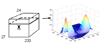
PARAFAC will decompose an array of order N (where N >= 3) into the summation over the outer product of N vectors (a low-rank model). E.g. if N=3 then the array is size I by J by K. An example of three-way fluorescence data is shown below..

For example, twenty-seven samples containing different amounts of dissolved hydroquinone, tryptophan, phenylalanine, and dopa are measured spectrofluoremetrically using 233 emission wavelengths (250-482 nm) and 24 excitation wavelengths (200-315 nm each 5 nm). A typical sample is also shown.

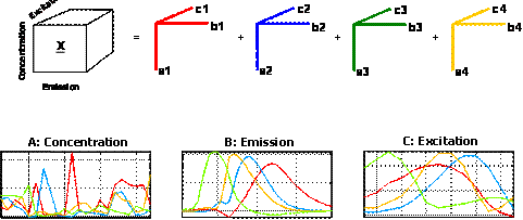
A four-component PARAFAC model of these data will give four factors, each corresponding to one of the chemical analytes. This is illustrated graphically below. The first mode scores (loadings in mode 1) in the matrix A (27x4) contain estimated relative concentrations of the four analytes in the 27 samples. The second mode loadings B (233x4) are estimated emission loadings and the third mode loadings C (24x4) are estimated excitation loadings.

For more information about how to use PARAFAC, see the University of Copenhagen's Multi-Way Analysis Videos.

In the PARAFAC algorithm, any missing values must be set to NaN or Inf and are then automatically handled by expectation maximization. This routine employs an alternating least squares (ALS) algorithm in combination with a line search. For 3-way data, the initial estimate of the loadings is usually obtained from the tri-linear decomposition (TLD).

For assistance in preparing batch data for use in PARAFAC please see bspcgui.

Inputs

• x = the multiway array to be decomposed, and

• ncomp =

• the number of factors (components) to use, OR
• a cell array of parameters such as {a,b,c} which will then be used as starting point for the model. The cell array must be the same length as the number of modes and element j contain the scores/loadings for that mode. If one cell element is empty, this mode is guessed based on the remaining modes.

Optional Inputs

• initval =

• If a parafac model is input, the data are fit to this model where the loadings for the first mode (scores) are estimated.
• If the loadings are input (e.g. model.loads) these are used as starting values.

• options = discussed below.

Outputs

The output model is a structure array with the following fields:

• modeltype: 'PARAFAC',

• datasource: structure array with information about input data,

• date: date of creation,

• time: time of creation,

• info: additional model information,

• loads: 1 by K cell array with model loadings for each mode/dimension,

• pred: cell array with model predictions for each input data block,

• tsqs: cell array with T² values for each mode,

• ssqresiduals: cell array with sum of squares residuals for each mode,

• description: cell array with text description of model, and

• detail: sub-structure with additional model details and results.

Note that the sum-squared captured table contains various statistics on the information captured by each component. Please see MCR and PARAFAC Variance Captured for details. The output pred is a structure array that contains the approximation of the data if the options field blockdetails is set to 'all' (see next).

Options

options = a structure array with the following fields:

• display: [ {'on'} | 'off' ], governs level of display,

• plots: [ {'final'} | 'all' | 'none' ], governs level of plotting,

• weights: [], used for fitting a weighted loss function (discussed below),

• stopcriteria: Structure defining when to stop iterations based on any one of four criteria

• relativechange: Default is 1e-6. When the relative change in fit gets below the threshold, the algorithm stops.
• absolutechange: Default is 1e-6. When the absolute change in fit gets below the threshold, the algorithm stops.
• iterations: Default is 10.000. When the number of iterations exceeds the threshold, the algorithm stops.
• seconds: Default is 3600 (seconds). When the time spent exceeds the threshold, the algorithm stops.

• init: [ 0 ], defines how parameters are initialized (discussed below),

• line: [ 0 | {1}] defines whether to use the line search {default uses it},

• algo: [ {'ALS'} | 'tld' | 'swatld' ] governs algorithm used. Only ALS allows more than three-way and allows constraints,

• iterative: settings for iterative reweighted least squares fitting (see help on weights below),

• scaletype: Defines how loadings are scaled. See options.scaletype.text for help,

• blockdetails: 'standard'

• preprocessing: {[]}, one element cell array containing preprocessing structure (see PREPROCESS) defining preprocessing to use on the x-block

• samplemode: [1], defines which mode should be considered the sample or object mode,

• constraints: {3x1 cell}, defines constraints on parameters (discussed below),

• coreconsist: [ {'on'} | 'off' ], governs calculation of core consistency (turning off may save time with large data sets and many components), and

• waitbar: [ {'on'} | 'off' ], display waitbar.

The default options can be retrieved using: options = parafac('options');.

Weights

Through the use of the options field weights it is possible to fit a PARAFAC model in a weighted least squares sense The input is an array of the same size as the input data X holding individual weights for each element. The PARAFAC model is then fit in a weighted least squares sense. Instead of minimizing the frobenius norm ||x-M||² where M is the PARAFAC model, the norm ||(x-M).*weights||² is minimized. The algorithm used for weighted regression is based on a majorization step according to Kiers, Psychometrika, 62, 251-266, 1997 which has the advantage of being computationally inexpensive. If alternatively, the field weights is set to 'iterative' then iteratively reweighted least squares fitting is used. The settings of this can be modified in the field iterative.cutoff_residuals which defines the cutoff for large residuals in terms of the number of robust standard deviations. The lower the number, the more subtle outliers will be ignored. The weights found during iterations can be found in model.detail.iteratively_found_weights but only of options.blockdetails has been set to 'all'.

Init

The options field init is used to govern how the initial guess for the loadings is obtained. If optional input initval is input then options.init is not used. The following choices for init are available.

Generally, options.init = 0, will do for well-behaved data whereas options.init = 10, will be suitable for difficult models. Difficult models are typically those with many components, with very correlated loadings, or models where there are indications that local minima are present.

• init = 0, PARAFAC chooses initialization {default},

• init = 1, uses TLD (unless there are missing values then random is used),

• init = 2, initializes loadings with random values,

• init = 3, based on orthogonalization of random values (preferred over 2),

• init = 4, based on singular value decomposition,

• init = 5, based on compression which may be useful for large data, and

• init > 5, based on best fit of many (the value options.init) small runs.

Constraints

The options field constraints is used to employ constraints on the parameters. It is a cell array with number of elements equal to the number of modes of the input data X. Each cell contains a structure array that defines the constraints in that particular mode. Hence, options.constraints{2} defines constraints on the second mode loadings. For help on setting constraints see constrainfit.

Examples

parafac demo gives a demonstration of the use of the PARAFAC algorithm.

model = parafac(X,5) fits a five-component PARAFAC model to the array X using default settings.

pred = parafac(Z,model) fits a parafac model to new data Z. The scores will be taken to be in the first mode, but you can change this by setting options.samplemodex to the mode which is the sample mode. Note, that the sample-mode dimension may be different for the old model and the new data, but all other dimensions must be the same.

options = parafac('options'); generates a set of default settings for PARAFAC. options.plots = 0; sets the plotting off.

options.init = 3; sets the initialization of PARAFAC to orthogonalized random numbers.

options.samplemodex = 2; Defines the second mode to be the sample-mode. Useful, for example, when fitting an existing model to new data has to provide the scores in the second mode.

model = parafac(X,2,options); fits a two-component PARAFAC model with the settings defined in options.

parafac io shows the I/O of the algorithm.

See Also

bspcgui, datahat, explode, gram, mpca, outerm, parafac2, preprocess, tld, tucker, unfoldm