Shapleygui

Introduction

Shapley Values are a game-theoretic approach to explaining an output from an objective function. In Chemometrics, one can use Shapley Values to understand how each variable additively contributes to a prediction. A popular tool for ExplainableAI, Shapley Values can help one understand the prediction behavior for any model type, including nonlinear models like ANN, ANNDL, SVM, and XGB.

To start the interface run the 'shapleygui' function from the Matlab command line:

shapleygui

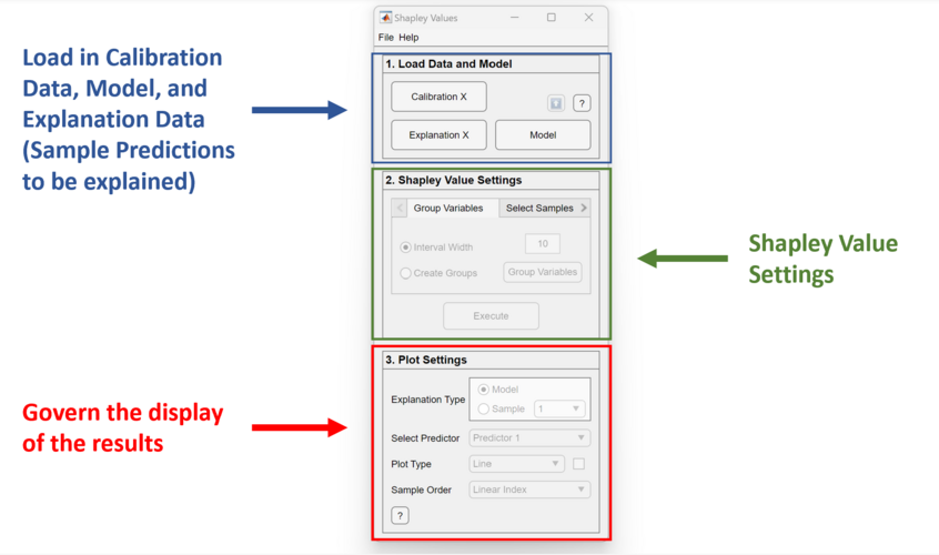
Shapley Values Interface

• Load Data and Model Panel

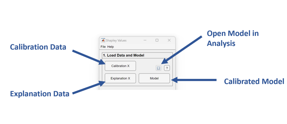
In this panel, one loads samples to be applied to the model. Shapley Values will be calculated to explain the predictions from those samples. One can load any model type for this application.

• Shapley Value Settings Panel

Define how the Shapley Value calculation will be done. For systems with > 500 variables, it is recommended to group the variables instead of doing Shapley for every variable. One can group variables by setting an interval width > 1, or by manually creating the groups.

• Plot Settings

View results. One can switch between overall model explanations or sample explanations. Switch between different predictors and plot types to discover trends of model predictions.

Load Data and Model

Shapley Values will explain a model's predictions from what's known as the 'Explanation X'. There is freedom in choosing the samples for this XBlock. One can use the calibration set, a subset of the calibration set, a class of samples from the calibration set, or validation data. Results might vary depending on what's chosen for these samples but should still fairly represent the model prediction behavior.

There will be Shapley Values for each of the outputs of a model. For example, if an M by N dataset was compressed to M X P by a UMAP model, then Shapley will return a M X N X P matrix. In the interface, one can see how the model predicts for each of the outputs by selecting the predictor in the Plot Settings description.

Shapley Value Settings

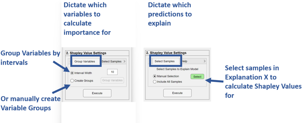
Through the interface, there are two things that need to be decided on, if Shapley Values are calculated for every variable or done on variable groups, and which samples from the explanation dataset will be used to explain the model.

Group Variables

Shapley Values can be done for every variable or done on groups of variables. To do Shapley Values on all variables, set the interval width to 1. One can group variables by setting an interval width > 1, or by manually creating the groups. For systems with > 500 variables, it is strongly encouraged to group the variables instead of doing Shapley for every variable. Grouping of variables can reduce the computation time significantly. For Shapley Values done on groups of variables, results will be in a lower resolution than if they were done on all variables, but can provide a simpler and perhaps more useful explanation.

Select Samples

There is freedom in choosing the samples for Explanation X. One can use the full calibration set, a subset of the calibration set, a class of samples from the calibration set, or validation data. Results might vary depending on what's chosen for these samples but should still fairly represent the model prediction behavior.

Plot Settings

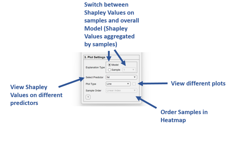
There are numerous settings and ways to explain predictions using Shapley Values. See each setting's description below.

Explanation Type

Shapley Values provide explanations for the predictions of each sample that is included in Explanation X. The Shapley Values for a sample summed with the base prediction will equal the prediction of that sample.

One can also aggregate Shapley Values to gain a general understanding of how the model predicts across all samples in Explanation X. There are numerous ways to aggregate this matrix. The most common way is to take the mean of the absolute value of the matrix, which is what's done in the software. For example, a M X N X P Shapley Value matrix will be aggregated to a 1 X N X P matrix. This type of aggregation can lend itself to a simpler explanation of the model since it will show if variables contribute significantly or not, either in the positive or negative direction.

Plot Type

Different plot types are available to help provide insight. See each plot type and their examples below.

Line, Line+Points, Scatter, Bar

These plot types provide a general explanation of the model by aggregating the Shapley Value matrix across the samples from the Explanation X for a particular predictor P. These plots show which variables are contributing significantly to the sample's prediction or not. Variables or variable groups that contribute significantly are good candidates for Variable Selection.

Heatmap

This plot type is an image of the Shapley Values for all of the sample's predictions on a particular predictor P. Each pixel is a sample and one of its variables and is colored by its Shapley Value, which indicates how much that variable individually contributed towards the sample's prediction. The sum of a sample's Shapley Values summed with the base prediction is equal to the sample's prediction. A subplot of the predictions is shown above. One can sort this image by the predictions on any Predictor P.

Beeswarm

This is a Scatter plot of all the sample's Shapley Values. If Shapley is done on all variables, then the samples will be colored by the response at that variable. Also, it may be useful to autoscale the colors if working with discrete data as opposed to spectra. If Shapley is done on variable groups, then they won't be colored by the data. If the number of variable/variable groups is 50 or less, then an XJitter will be added to show the density of samples with the same Shapley Values.

Sample Order

Only applicable to the Heatmap plot. Select between different predictors to sort the samples in the Heatmap and Prediction plot.

Saving Results

The results from the calculation can be saved to the workspace or a .mat file. One can do this by clicking on the Save button. One can also save the variables that have the highest magnitude of Shapley for a predictor P. One can do this by right-clicking in the plot and selecting 'Save Variables with Highest Shapley'. One will then be prompted to provide a number of top variables/variable groups to save. Once this number is provided, one can then save the vector of variables with the highest Shapley on that predictor P, lending it to do Variable Selection.