Genetic Algorithms for Variable Selection

Introduction

Genetic algorithm variable selection is a technique that helps identify a subset of the measured variables that are, for a given problem, the most useful for a precise and accurate regression model. The earlier discussion of multivariate regression describes how multiple variables can be used together to better predict a separate quantity and how the expected relationship between the measured variables can be used to identify outliers and other faults (through Q residuals and Hotelling's T2). Many regression problems benefit from the multivariate advantages of more precise predictions and outlier detection. In some cases, however, some variables may be expensive or difficult to measure (expensive variables) and others may contain noise or interfering signal which may actually deteriorate the accuracy and/or precision of a regression model (noisy variables). In these cases, it can be advantageous to discard some variables.

Noisy variables can sometimes be identified with knowledge of the measurement technique being used. If a given sensor is known to be highly susceptible to noise and/or responds very little to the changes of interest in a system, it can often be discarded. Similarly, spectral data often include regions in which the instrumentation has very poor sensitivity and the species of interest have little to no response. These regions can often be discarded, thus improving a model. Sometimes, however, the choice of what variables to discard is not as clear.

Expensive variables pose a similar dilemma. Although many variables may be of use in a prediction, time, money, or other engineering considerations may preclude measuring all the variables originally considered for a regression model. In these cases, it is useful to identify a subset of the variables that allows sufficient prediction accuracy and precision while minimizing the number of variables to be measured.

Although there are a variety of variable selection methods, genetic algorithms (GA) provide a straightforward method based on a "survival of the fittest" approach to modeling data.

Genetic Algorithm Theory

Given an X-block of predictor data and a Y-block of values to be predicted, one can choose a random subset of variables from X and, through the use of cross-validation and any of the regression methods described earlier, determine the root-mean-square error of cross validation (RMSECV) obtained when using only that subset of variables in a regression model. Genetic algorithms use this approach iteratively to locate the variable subset (or subsets) which gives the lowest RMSECV.

The first step of the GA is to generate a large number (e.g., 32, 64, 128) of random selections of the variables and calculate the RMSECV for each of the given subsets. When using factor-based regression methods (e.g., PLS) the maximum number of allowed factors in a model is limited, and the RMSECV used is the lowest obtained using up to that limit.

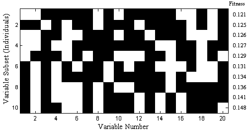
Each subset of variables is called an individual and the yes/no flags indicating which variables are used by that individual is the gene for that individual. The pool of all tested individuals is the population. The RMSECV values, described as the fitness of the individual, indicate how predictive each individual's selection of variables is for the Yblock. Because of varying levels of noise and interference in the variables, the fitness of the different individuals in the population will extend over some range of values. Figure 1 shows ten out of a total of 64 variable subsets and resultant RMSECV values for the slurry-fed ceramic melter data.

Figure 1. Map of example of selected variables for 10 of 64 individuals (white square indicates a selected variable)

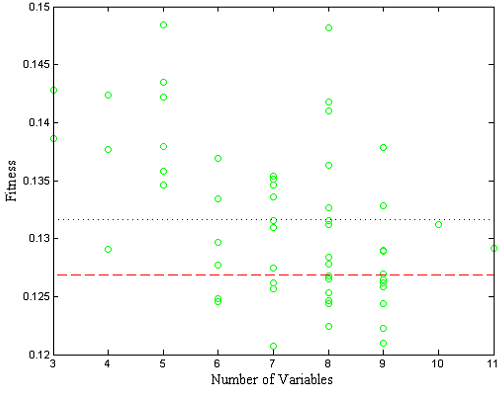
The RMSECV results for all of the individuals can also be examined as a function of the number of included variables. Figure 2 shows the results obtained from an example population for the SFCM data. Also shown is the median of all individual RMSECV fits (dotted line) and the RMSECV obtained using all the variables (dashed line). Note that at this point, many of the individuals performed worse than when all the variables were used.

Figure 2. Fitness (RMSECV) versus the number of variables used by each individual.

The second step in the GA is selection. The individuals with fitness greater than the median fitness (i.e., all models above the dotted line in Figure 2) are discarded. The remaining individuals used variables which, for one reason or another, provided a lower RMSECV – a better fit to the data. At this point, the population has been shrunk to half its original size. To replace the discarded individuals, the GA "breeds" the retained individuals.

In PLS_Toolbox, breeding is done by one of two methods: single or double cross-over. In single cross-over, the genes from two random individuals are split at some random point in the gene. The first part of the gene from individual A is swapped with the first part of the gene from individual B, and the two hybrid genes form two new individuals (C and D) for the population. This is shown schematically in Figure 3. Double cross-over breeding (also shown in the figure) is very similar to single cross-over except that two random points in the gene are selected and the middle portions of the two genes are swapped. The biggest practical difference is that double cross-over usually produces new individuals with less change from the original parent genes. Put in terms of selected variables, double cross-over typically creates new variable subsets which more-closely match the variables included in one parent or the other.

Figure 3. Schematic of single and double cross-over breeding.

After adding the new individuals to the population, all the individuals' genes are given a chance for random mutation. This allows for a finite chance of adding or removing the use of variables that might be over- or under-represented in the population (See variable 13 in Figure 1 for an example of an underrepresented variable).

Finally, after all the individuals have been paired and bred, the population returns to the original size and the process can continue again at the fitness evaluation step. The entire process is:

1. Generate random variable subsets
2. Evaluate each individual subset of selected variables for fitness to predict Y
3. Discard worse half of individuals
4. Breed remaining individuals
5. Allow for mutation
6. Repeat steps 2-5 until ending criteria are met

The GA will finish (a) after a finite number of iterations or (b) after some percentage of the individuals in the population are using identical variable subsets. Individuals using noisy variables will tend to be discarded; thus, the variables used by those individuals will become less represented in the overall gene population. Likewise, less noisy variables will become more and more represented. Depending on the number of variables and the rate of mutation, many of the individuals will eventually contain the same genes.

Practical GA Considerations

One of the biggest risks in GA variable selection is over-fitting. It is possible that the variables selected may be particularly good for generating a model for the given data, but may not be useful for future data. This is particularly problematic when analyzing data with smaller numbers of samples. Although the GA uses a modified version of cross-validation to help avoid this (see below), it is generally recommended that these guidelines be followed:

1. Keep the ending criteria sensitive. The more iterations which occur, the more feedback the GA will have from the cross-validation information, and thus the more likely the over-fitting,
2. Use random cross-validation and multiple iterations if practical,
3. Repeat the GA run multiple times and watch for general trends, and
4. When analyzing data with many variables and fewer samples (short-fat problems), set the window width (see below) to a larger value to use blocks of variables and keep the maximum number of latent variables low.

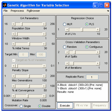
In Solo, genetic algorithm variable selection is performed using the Genetic Algorithm Window. In PLS_Toolbox, genetic algorithm variable selection is performed using one of two functions, the Genetic Algorithm Window (genalg), or the command-line version (gaselctr). If genalg is used, data must first be loaded using the File/Load Data menu. If any preprocessing should be used, this can be set using the Preprocess menu. In either the window-based or the command-line routine is used, various GA settings need to be specified. In the the GA Window, these settings are selected using graphical controls (see Figure 4); in the command-line interface, the settings are selected via an options structure. The following describes the settings and gives the name of the appropriate options field in parenthesis.

Figure 4. GUI interface used to specify GA settings.

• Size of Population (popsize) – The larger the population size, the more time required for each iteration. Larger populations do, however, provide a better representation of different variable combinations. One alternative to using a large population size is to use multiple replicate runs (reps); this, however, does not allow for interbreeding between potentially useful gene mixtures.

• Window Width (windowwidth) – When adjacent variables contain correlated information, or the end use of the variable selection is to include or exclude adjacent variables together as a block (e.g., lower-resolution measurement), the original variables can be grouped together and included or excluded in "blocks". Window width indicates how many adjacent variables should be grouped together at a time. The grouping starts with the first variable and the subsequent (windowwidth-1) variables.

• % Initial Terms (initialterms) – Specifies the approximate number of variables (terms) included in the initial variable subsets. Starting with fewer initial terms will make the identification of useful variables more difficult, but will bias the end solution towards models with fewer variables. See also Target.

• Target Min/Max (target) and Penalty slope (penaltyslope) – These settings are used together to guide the algorithm towards a solution with a given number (or percentage) of included variables. To use this feature, first set some level of penalty slope to enable the Target Min/Max edit boxes. Prior to discarding the unfit individuals, each individual is tested for the total number of variables used. Any individual using more variables than the Target Max or less than the Target Min will be penalized by increasing the RMSECV fitness, based on the number of variables above or below the limits times the penalty slope:

RMSECV ′ = RMSECV(1+ρn)

where ρ is the penalty slope and n is the number of variables the individual used above or below the target range. The result is that an individual with a good fit but using too many or too few variables will be more likely to be discarded, unless the fit is unusually better than that of other individuals. In the GA Window, the penalty slope must first be selected, then the target range.

Target range can be specified in absolute number of variables or in percentage of total variables, based on the % checkbox to the right of the target. In the options structure, the percentage is specified using the targetpct field. A value of 1 (a checked checkbox in the GA Window) indicates that target is specified in percent.

• Max Generations (maxgenerations) and Percent at Convergence (convergence) – Specify the ending criteria as described earlier. Lower settings for both will help avoid over-fitting of data. It is sometimes useful to perform many replicate runs with a lower setting for maximum generations.

• Mutation rate (mutationrate) – The higher the mutation rate, the more chance of including underrepresented variables or excluding over-represented variables.

• Regression Choice (algorithm) and # of LVs (ncomp) – Specifies the regression method as MLR (use all selected variables) or PLS (use latent variables derived from selected variables). The number of LVs slider (or ncomp option) specifies the maximum number of latent variables which can be used in a PLS model. This should generally be kept near the number of LVs necessary to accurately model the data and should be no more than absolutely necessary (to avoid overfitting).

• Cross-Validation settings (cv, split, iter) – Selects the type and number of splits and iterations to be used for cross-validation. Note that the contiguous block cross-validation used by GA is slightly modified from that used in standard cross-validation. Although the samples are still selected and left-out in contiguous blocks, the starting position of the first block shifts randomly through the data. This helps reduce the likelihood of over-fitting.

• Replicate Runs (reps) – This specifies the number of times the GA should be run using the specified conditions. The results of each cycle will be concatenated together and will appear together in the results plots, as described below.

The settings can be saved from the GA Window for use as an options structure in the command line function by selecting File/Save Settings and specifying a variable to which the options should be saved.

After the settings have been specified as desired, the analysis can be started in the GA Window by selecting Execute. From the command line, executing gaselctr will start the analysis with the given settings:

gaselctr(x,y,options)

Analysis of GA Results

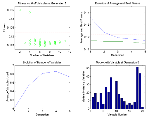
During the analysis, a four-plot figure will be provided and the command window will display the progress of the GA run. An example is shown in Figure 5. The top left plot indicates the fitness vs. number of included variables for each member of the current population. The RMSECV obtained using all variables will be shown as a dashed horizontal line. If target and penalty slope are being used, the penalized fitness will be shown as red dots along with the actual fitness as the usual green circles.

The top right plot shows the trend of the average fitness (top line) and the best fitness (bottom line) with generation number. The horizontal dashed line is the RMSECV obtained using all variables. The best fitness represents how well the best model is doing. As the population begins to become more similar, the best and average fitness lines converge. If neither line is changing much, the GA has either reached a consensus of selected variables or the equivalent solutions with different selected variables.

The bottom right plot shows the change with each generation in the average number of variables used by each individual in the population. When min/max targets are not being used, this plot shows the natural trend towards some number of required variables. With min/max targeting, the plot indicates how well the target is being met, on average.

The bottom left plot indicates the total number of times each variable is used in the population. Variables which are used more are usually more useful in the regression.

Variables which show up less are less useful. Note, however, that depending on the population size, mutation rate, and total number of generations, the frequency of inclusion of any given variable may be biased. It is best to compare frequency of usage with multiple replicates or large, young populations.

Figure 5. Example of diagnostic plots shown during GA run.

It is generally true that the entire set of selected variables should be considered as a whole as opposed to considering each variable as useful on its own. This is because a variable may only be helpful to prediction when used in conjunction with other variables included in an individual variable subset.

Once the analysis is done, two additional plot buttons will be available on the GA Window: Fit vs. Var (Fitness versus Number of Variables) and Frequency. These two buttons return results similar to the top left and bottom right plots, respectively, in Figure 5. However, they include the compiled results from all replicate runs.

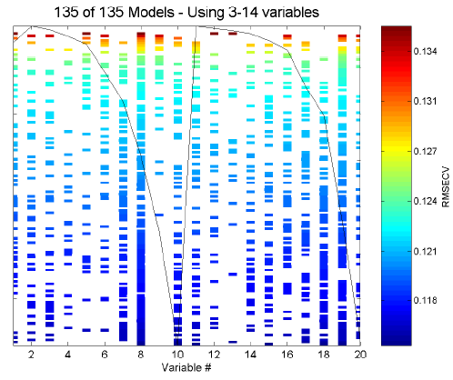
Fit vs. Var includes some additional information and can be used to look for trends in variable usage. Initially, you are presented with a plot of fitness of each individual versus the number of included variables. Use the mouse to select some range of the individuals (for example, if you wish to examine only models using more variables, select only these individuals from the plot). Next, a plot indicating variable usage, color coded by resulting RMSECV, will be shown. For reference, the mean of the raw data is overlaid on the plot of included variables. Figure 6 shows an example of a Fit vs. Var variable usage plot for the SFCM data.

Figure 6. Example of Fit vs. Var plot for SFCM data.

The variable usage plot is most useful to identify trends. If inclusion of a given variable tends to improve the RMSECV, the inclusion marks for this variable will tend to appear towards the bottom of the figure. Conversely, a variable which tends to degrade the RMSECV will tend to appear towards the top of the figure. If a variable doesn't show up at all, it is likely to be not useful and if it is used in all the models, it is probably more useful.

It is very important, however, to consider the range of RMSECVs observed through the models. In many cases, the final RMSECV values will be very similar for the individual models, and, as such, the differences in selected variables are not important. If, however, the GA run is stopped early, when a large range in RMSECV exists, more general trends can be observed. Figure 6, for example, shows the results of 135 models after only three generations. It can be clearly seen that variable 9 is harmful to good RMSECV while variable 11 is not useful but not harmful.

Figure 7. Example of Fit vs. Var plot for NIR spectra of simulated gasoline.

A second example of fit as a function of variables-used is shown in Figure 7. The X-block is the spec1 dataset in the nir_data.mat file and the Y-block is the first column of the conc dataset. For this run, the window width was set to 25 variables, the maximum number of latent variables was set at five, and the analysis was repeated for a total of six replicate runs; otherwise, all other settings were at their default value.

Note that the RMSECV covers a fairly large range from just under 0.3% (absolute error in concentration as weight/weight %) to just above 0.6%, so the worst of these models are twice as bad as the best models at predicting the concentration. Nearly all models use the windows of variables centered at 138, 263, 288, and 388. Very few models, and almost none of the best models, use variables at 38, 63, 88, 138, 188, or 338. These variable windows are either not useful or are actually detrimental to the prediction of the concentration of this component. It can be seen that the selected regions fall on or near the spectral peaks of the mean spectrum, overlaid for reference on the plot.

Once a GA run is complete, the X-block data can be re-saved with only the selected variables (those used for the model with lowest RMSECV). The menu option File/Save Best/as Dataset will save the X-block data with the include field set to only the selected variables. To save only the selected variables as a standard array (i.e., not in DataSet Object format), use File/Save Best/as Matrix. This will save only the selected variables of the data as a simple array object. Either of these can be read into the Analysis Window and used in further modeling.

The results and statistics of the GA run can also be saved as a structure by selecting File/Save Results and specifying a variable name. This structure contains various fields including the RMSECV for each final model in the rmsecv field, and the variables selected for each of those models as a binary representation (1 = selected) in the icol field. The first row of icol corresponds to the first entry in rmsecv.