Svmda

Purpose

SVMDA Support Vector Machine (LIBSVM) for classification. Use SVM for support vector machine regression(Svm).

Synopsis

model = svmda(x,options); %identifies model (calibration step) based on x-block classes

model = svmda(x,y,options); %identifies model (calibration step)

pred = svmda(x,model,options); %makes predictions with a new X-block

pred = svmda(x,y,model,options); %performs a "test" call with a new X-block and known y-values

Description

SVMDA performs calibration and application of Support Vector Machine (SVM) classification models. (Please see the svm function for support vector machine regression problems). These are non-linear models which can be used for classification problems. The model consists of a number of support vectors (essentially samples selected from the calibration set) and non-linear model coefficients which define the non-linear mapping of variables in the input x-block. The model allows prediction of the classification based on either the classes field of the calibration x-block or a y-block which contains integer-valued classes. It is recommended that regression be done through the svm function.

Svmda is implemented using the LIBSVM package which provides both cost-support vector regression (C-SVC) and nu-support vector regression (nu-SVC). Linear and Gaussian Radial Basis Function kernel types are supported by this function.

Note: Calling svmda with no inputs starts the graphical user interface (GUI) for this analysis method.

Inputs

• x = X-block (predictor block) class "double" or "dataset", containing numeric values,
• y = Y-block (predicted block) class "double" or "dataset", containing integer values,
• model = previously generated model (when applying model to new data).

Outputs

• model = a standard model structure model with the following fields (see Standard Model Structure):
  • modeltype: 'SVM',
  • datasource: structure array with information about input data,
  • date: date of creation,
  • time: time of creation,
  • info: additional model information,
  • pred: 2 element cell array with
    • model predictions for each input block (when options.blockdetail='normal' x-block predictions are not saved),
  • classification: information about the classification of X-block samples (see description at Standard Model). For more information on class predictions, see Sample Classification Predictions.,
  • detail: sub-structure with additional model details and results, including:
    • model.detail.svm.model: Matlab version of the libsvm svm_model (Java). Note that the number of support vectors used is given by model.detai.svm.model.l. It is useful to check this because it can indicate overfitting if most of the calibration samples are used as support vectors, or can indicate problems fitting a model if there are no support vectors (and all prediction values will equal a constant value, a weighted mean).
    • model.detail.svm.cvscan: results of CV parameter scan
    • model.detail.svm.svindices: Indices of X-block samples which are support vectors.

• pred a structure, similar to model for the new data.
  • pred: The vector pred.pred{2} will contain the class predictions for each sample.

For more information on class predictions, see Sample Classification Predictions

Options

options = a structure array with the following fields:

• display: [ 'off' | {'on'} ], governs level of display to command window,
• plots [ 'none' | {'final'} ], governs level of plotting,
• classset [ {1} ], indicates which class set in x to use when no y-block is provided,
• preprocessing: {[]} preprocessing structures for x block (see PREPROCESS). NOTE that y-block preprocessing is NOT used with SVMDA. Any y-preprocessing will be ignored.
• compression: [{'none'}| 'pca' | 'pls' ] type of data compression to perform on the x-block prior to calculaing or applying the SVM model. 'pca' uses a simple PCA model to compress the information. 'pls' uses either a pls or plsda model (depending on the svmtype). Compression can make the SVM more stable and less prone to overfitting.
• compressncomp: [1] Number of latent variables (or principal components to include in the compression model.
• blockdetails: [ {'standard'} | 'all' ], extent of predictions and residuals included in model, 'standard' = only y-block, 'all' x- and y-blocks.
• algorithm: [ 'libsvm' ] algorithm to use. libsvm is default and currently only option.
• kerneltype: [ 'linear' | {'rbf'} ], SVM kernel to use. 'rbf' is default.
• svmtype: [ {'c-svc'} | 'nu-svc' ] Type of SVM to apply. The default is 'c-svc' for classification.
• probabilityestimates: [0| {1} ], whether to train the SVR model for probability estimates, 0 or 1 (default 1)"

• cvtimelimit: Set a time limit (seconds) on individual cross-validation sub-calculation when searching over supplied SVM parameter ranges for optimal parameters. Only relevant if parameter ranges are used for SVM parameters such as cost, epsilon, gamma or nu. Default is 10 (seconds);
• splits: Number of subsets to divide data into when applying n-fold cross validation. Default is 5. This option is only used when the "cvi" option is empty.
• cvi: {{}} Standard cross-validation cell (see crossval) defining a split method, number of splits, and number of iterations. This cross-validation is use both for parameter optimization and for error estimate on the final selected parameter values. If empty (the default), then random cross-validation is done based on the "splits" option.
• gamma: Value(s) to use for LIBSVM kernel gamma parameter. Default is 15 values from 10^-6 to 10, spaced uniformly in log.
• cost: Value(s) to use for LIBSVM 'c' parameter. Default is 11 values from 10^-3 to 100, spaced uniformly in log.
• nu: Value(s) to use for LIBSVM 'n' parameter (nu of nu-SVC, and nu-SVR). Default is the set of values [0.2, 0.5, 0.8].
• strictthreshold: Probability threshold value to use in strict class assignment, see Sample_Classification_Predictions#Class_Pred_Strict. Default = 0.5.

Algorithm

Svmda uses the LIBSVM implementation using the user-specified values for the LIBSVM parameters (see options above). See [1] for further details of these options.

The default SVMDA parameters cost, nu and gamma have value ranges rather than single values. This svm function uses a search over the grid of appropriate parameters using cross-validation to select the optimal SVM parameter values and builds an SVM model using those values. This is the recommended usage. The user can avoid this grid-search by passing in single values for these parameters, however.

Model building performance

Building a single SVM model can sometimes be slow, especially if the calibration dataset is large. Using ranges for the SVM parameters to search for the optimal parameter combination increases the final model building time significantly. If cross-validation is used the calculation is again increased, possibly dramatically if the number of CV subsets is large. Some suggestions for faster SVM building include:

1) Turning CV off ("none") during preliminary analyses. This is MUCH faster and cross-validation is still performed using a default "Random Subsets" with 5 data splits and 1 iteration,

2) Using a coarse grid of SVM parameter values to search over for optimal values,

3) Choosing the CV method carefully, at least initially. For example, use "Random Subsets" with a small number of data splits (e.g. 5) and a small "Number of Iterations" (e.g. 1).

4) Using the compression option if the number of variables is large.

C-SVC and nu-SVC

There are two commonly used versions of SVM classification, 'C-SVC' and 'nu-SVC'. The original SVM formulations for Classification (SVC) used parameter C, [0, inf), to apply a penalty to the optimization for data points which were not correctly separated by the classifying hyperplane. An alternative version of SVM classification was later developed where the C penalty parameter was replaced by a nu, [0,1], parameter which applies a slightly different penalty. The main motivation for the nu version of SVM is that it has a has a more meaningful interpretation because nu represents an upper bound on the fraction of training samples which are errors (misclassified) and a lower bound on the fraction of samples which are support vectors. Some users feel nu is more intuitive to use than C. C and nu are just different versions of the penalty parameter. The same optimization problem is solved in either case. Thus it should not matter which form of SVM you use, C versus nu for classification. PLS_Toolbox uses the C version by default since this was the original formulation and is the most commonly used form. For more details on 'nu' SVMs see [2]

The user must provide parameters (or parameter ranges) for SVM classification as:

• 'C-SVC':

C, (using linear kernel), or

C, gamma (using radial basis function kernel),

• 'nu-SVC':

nu, (using linear kernel), or

nu, gamma (using radial basis function kernel),

Class prediction probabilities

LIBSVM calculates the probabilities of each sample belonging to each possible class if the "Probability Estimates" option is enabled (default setting) in the SVMDA analysis window (or if the probabilityestimates option is set equal to 1 (default value) in command line usage). The method is explained in [3], section 8, "Probability Estimates". PLS_Toolbox provides these probability estimates in model.detail.predprobability or predict.detail.predprobability, which are nsample x nclasses arrays. The columns are the classes, in the order given by model.detail.svm.model.label (or prediction.detail.svm.model.label), where the class values are what was in the input X-block.class{1} or Y-block. These probabilities are used to find the most likely class for each sample and this is saved in pred.pred{2} and model.detail.predictedclass. This is a vector of length equal to the number of samples with values equal to class values (model.detail.class{1}).

SVMDA Parameters

• cost: Cost [0 ->inf] represents the penalty associated with errors. Error refers to a sample which do not lie on the proper side of the margin for that sample's class. Increasing cost value causes closer fitting to the calibration/training data and usually a narrower margin width. nu is not required if cost is specified.
• gamma: Kernel gamma parameter controls the shape of the separating hyperplane. Increasing gamma usually increases number of support vectors.
• nu: Nu (0 -> 1] is an alternative parameter for specifying the penalty associated with errors. It indicates a lower bound on the number of support vectors to use, given as a fraction of total calibration samples, and an upper bound on the fraction of training samples which are errors (misclassified). cost is not required if nu is specified. There is a constraint on the nu parameter, however, related to the number of training data points in each class. For every class pair, having n1 and n2 data points each, nu must be less than 2*min(n1, n2)/(n1+n2), i.e. nu must be less than the ratio of the smaller class count to the pair average class count. SVMDA automatically checks for this possibility in nu-svc.

Examples of SVMDA models on simple two-class data

Users of SVMs will usually not pick the values for their SVM parameters cost/nu and gamma because there is no simple way to know what values would provide a good model for their data. Instead, they should search over parameter ranges testing SVM models to find which parameter combination works best for their data, as discussed below. However, it is still a good idea to have an idea of how these parameters affect how the SVM works on their data. For this reason we look here at the effects of cost/nu and gamma on a very simple dataset, an x-block of two variables where the data belong to just two classes, to allow visualization of the optimal separating boundary. In practice the user will usually work with multivariate x-block data having more than two variables and data belonging to multiple classes, so will only view the predicted classes versus actual classes and related skill measures, and some details such as the number of support vectors involved.

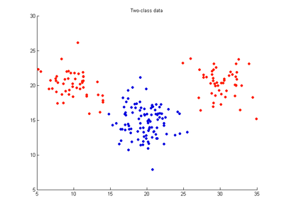
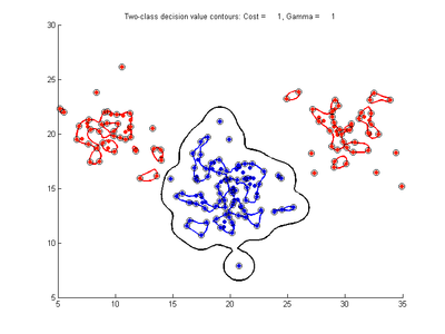
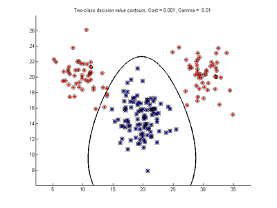
The effects of the cost, gamma and nu parameters on SVMDA are examined by applying SVMDA to a simple two-variable (x1,x2) dataset where 100 samples belong to red class and 100 to blue class. This is equivalent to an X-block having dimensions 200x2. The data are distributed as three clusters, two red clusters with 50 points each which lie nearly on either side of a blue cluster which has 100 points. SVMDA attempts to draw a dividing line between these clusters separating the x1 vs x2 domain into red and blue regions. It uses these calibration data points to find the optimal separating decision boundary (hyperplane) with the widest separating margin. Any future test samples will be classified as red or blue according to which side of the separating boundary they occur on. The following images show SVMDA classification models trained on these data using an RBF kernel and varying values for the cost, gamma and nu parameters. Note that an SVMDA model with linear kernel cannot be a good model for this dataset since the red and blue points cannot be separated by a straight line, linear boundary.

• Fig. 1. Two-class dataset
• 

  Two-variable data with 100 red samples and 100 blue samples.

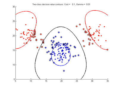
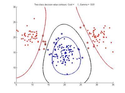
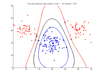
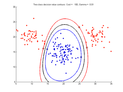
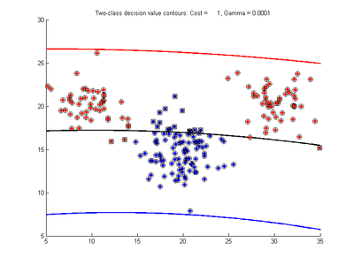
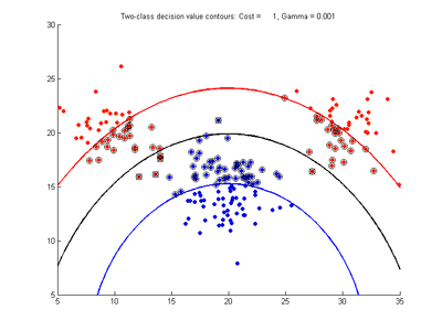
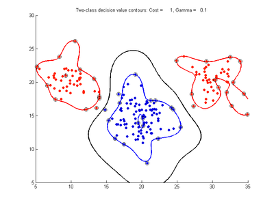
The figures below show results for various SVMDA models built on the simple dataset. They are presented with the decision boundary shown as a black contour line, the margin edges shown by blue and red contours, data points which are support vectors marked by an enclosing circle, and data points which lie on the wrong side of the decision boundary (classification errors) marked with an 'x'. The decision boundary represents the zero contour of the decision function, blue and red margin edges represent the -1 and +1 contours of the decision function.

Effect of varying cost parameter for SVMDA using RBF kernel

Fig. 2a-d show the effect of increasing the cost parameter from 0.1 to 100 while gamma is kept fixed = 0.01. When the cost is small. Fig. 2a, the margin is wide since there is a small penalty associated with data points which are within the margin. Note that any point which lies within the margin or on the wrong side of the decision boundary is a support vector. Increasing the cost parameter leads to a narrowing of the margin width and fewer data points remaining within the margin, until cost = 100 (Fig. 1d) where the margin is narrow enough to avoid having any points remain inside it. Further increases in cost have no effect on the margin since no data points remain to be penalized. At the other extreme, when cost is reduced to 0.01 or smaller, the margin expands until it encloses all the data points, so all points are support vectors. This is undesirable since fewer support vectors make a more efficient model when predicting for new data points and reduces the chance of overfitting the data. In this simple case, the separating boundary in all these cases keeps approximately the same smooth contour as in Fig. 2a, so overfitting is not an issue. If there was more overlapping of the red and greed data points then larger cost parameter would cause the separating boundary to deform slightly and the margin edges to be much more contorted as it tries to exclude data points from the margin.

• Fig. 2. Effect of varying cost parameter, with gamma = 0.01
• 

  a) cost = 0.1

• 

  b) cost = 1.0

• 

  c) cost = 10

• 

  d) cost = 100

Effect of varying gamma parameter for SVMDA using RBF kernel

Fig. 3a-f show the effect of changing the gamma parameter while cost is held fixed at 1.0. These show that gamma has a major effect on how smooth or contorted the decision boundary will be, with smaller values of gamma creating a smoother decision boundary. Fig3a shows the decision boundary to be nearly linear, showing that the SVM with RBF kernel tends to the linear kernel solution for gamma values tending towards zero. At large gamma values, however, the decision boundary becomes more contorted and shows how the SVM can over-fit the calibration data. The SVM in Fig. 3f produces a decision boundary which would not be a very good class predictor for the class of new test data samples.

• Fig. 3. Effect of varying gamma parameter, with cost = 1.0
• 

  a) gamma = 0.0001

• 

  b) gamma = 0.001

• 

  c) gamma = 0.01

• 

  d) gamma = 0.1

• 

  e) gamma = 1.0

• 

  f) gamma = 10.0

In summary, these comparisons show that the gamma parameter controls how smooth the decision boundary will be, with larger gamma producing more complicated boundaries, while the cost parameter controls the width of the separating margin, with larger values of cost making the margin narrower. They both affect the location of the decision boundary.

Effect of varying nu parameter for SVMDA using RBF kernel

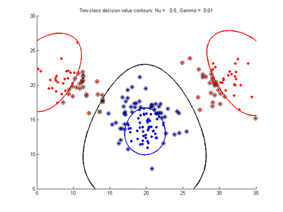
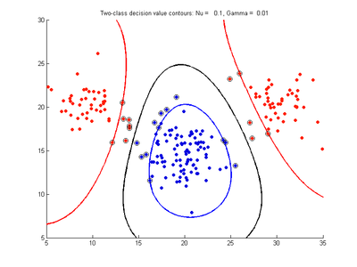
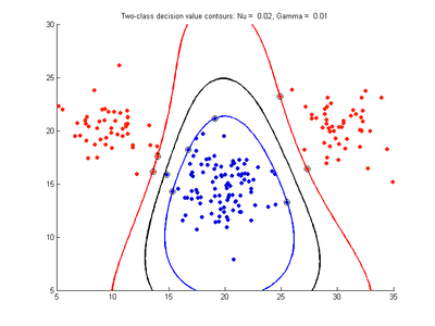
Fig. 4a-d show the effect of decreasing the nu parameter from 0.5 to 0.01 while gamma is kept fixed = 0.01. These figures show that decreasing nu has the same effect as was obtained by increasing the cost parameter, that is, it causes the margin width to decrease. It shows how nu is simply a different representation of the cost penalty parameter, and for any value of nu there is a corresponding value of cost which produces the same SVM. The reason for its use is that its value can be interpreted as a lower bound on the number of samples which are support vectors, and also as an upper bound on the number of misclassification errors.

• Fig. 4. Effect of varying nu parameter, with gamma = 0.01
• 

  a) nu= 0.5

• 

  b) nu = 0.1

• 

  c) nu = 0.02

• 

  d) nu = 0.01

Table 1. Compare nu value to SV fraction

nu value	SV fraction	number of SVs
0.5	0.505	101
0.1	0.105	24
0.02	0.045	9
0.01	0.020	4

Table 1 shows how the value of nu is a lower bound on the support vector fraction (number of SV/200), and an upper bound on the fraction of training samples which are errors (misclassified) for the SVMs in Fig. 4. The upper bound on the fraction of misclassification is easily satisfied here because the only misclassifications were three datapoints in Fig.4a.

Choosing the best SVM parameters

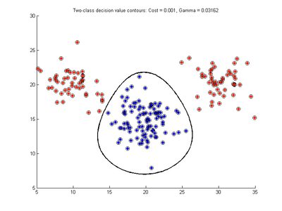
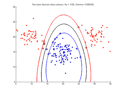
The recommended technique is to repeatedly test SVMDA using different parameter values and select the parameter combination which gives the best results. For SVMDA using c-svc/nu-svc and an RBF kernel we select ranges of the c/nu and gamma parameters, choosing equi-spaced (or equi-spaced in log) parameters over the ranges. SVMDA using c-svc uses 9 values of c between 0.001 and 100, and 9 values of gamma between 10^-6 and 10 by default, then tests each of these 81 pair combinations. Each test builds a c-svc model on the calibration data using 5-fold cross-validation to produce a mis-classification rate result for that test. These tests are compared over all 81 tests to find which cost/gamma value combination gives the best cross-validation prediction (smallest mis-classification). A similar approach is used for nu-svc where values of nu and gamma are specified. The results for the best model when using the simple data in Fig. 1 are shown here in Fig. 5 for the c-svc and nu-svc cases. These models were selected by searching over the default parameter ranges for the optimal model. Note, the nu parameter range was extended to smaller values than the default nu range, to include 0.05 and 0.1.

• Fig. 5. Optimal SVMDA models for c-svc and nu-svc
• 

  a) Optimal c-svc model. cost = 0.001, gamma = 0.03

• 

  b) Optimal nu-svc model. nu = 0.05, gamma = 0.003

The c-svc case in Fig. 5a has a very small cost parameter and all data points are support vectors. The decision boundary looks appropriate but this is not a good solution because of the large support vector fraction. Using an SVM to predict the class of a new sample involves calculating a sum over as many terms as there are support vectors. Thus a SVM with fewer support vectors will be faster when predicting the class of a new sample. Thus it would be good to limit the lower end of the cost parameter range to 0.1 perhaps. It should also be noted that SVMDA can have problems when using very small cost parameter (or nu very close to 1) while requesting probability estimates as this can result in bad model predictions for sample class. This problem does not arise when probability estimates are not requested. The next section discusses this problem in more detail. Note that all the models presented in Figs 1-5 were built with probability estimates disabled. Thus predictions are directly given by which side of the decision boundary the data points lie on.

SVM parameter search summary plot

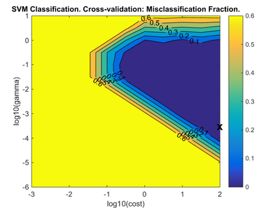
When SVMDA is run in the Analysis window it is possible to view the results of the SVM parameter search by clicking on the "Variance Captured" plot icon in the toolbar. If there are two SVM parameters with ranges of values, such as cost and gamma, then a figure appears showing the performance of the model plotted against cost and gamma (Fig. 6). The measure of performance used is the misclassification rate, defined as the number of incorrectly classified samples divided by the number of classified samples, based on the cross-validation (CV) predictions for the calibration data. The lowest value of misclassification rate is marked on the plot by an "X" and this indicates the values of the SVM cost and gamma parameters which yield the best performing model. The actual SVMDA model is built using these parameter values. If you are using the command line SVMDA function to build a model then the optimal SVM parameters are shown in model.detail.svm.cvscan.best. If you are using the graphical Analysis SVMDA then the optimal parameters are reported in the summary window which is shown when you mouse-over the model icon, once the model is built.

• Fig. 6. Parameter search summary
• 

  CV misclassification rate as a function of SVM parameters.

Possible poor prediction from the optimal SVM model

In support vector classification (SVC) the LIBSVM package allows classification predictions to be derived two different ways.

1. The standard method it to calculate the decision function for the new sample and simply assign the class label according to the sign of the decision function (in the case of two-class data). This is equivalent to saying the sample's class is determined by which side of the decision boundary it occurs on.

2. The second method to predict the class of a new sample was developed in order to also provide probabilities of the sample belonging to each possible class ([4], section 8, "Probability Estimates"). In this method the new sample is assigned to the class for which it has the highest probability of belonging to.

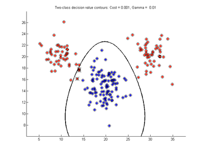
These two prediction methods produce nearly identical predicted class values but in certain cases there are noticeable differences. Test samples which lie very close to the decision boundary on the +1 side, for example, can be given a predicted class by the second method which identifies them incorrectly as the -1 class. This discrepancy between the two prediction methods becomes most noticeable when the SVM margin becomes very wide and encloses most data points (which are then support vectors). For the simple two-class data used here this is illustrated by comparing the two prediction methods using any gamma value but with a small very small cost (or large nu) parameter in Fig. 7 below, where again the color indicates the actual class of data points and a superimposed x indicates the predicted class is incorrect for that point. The decision boundary looks reasonable and the simpler method of identifying class by which side of the decision boundary samples occur on gives good predictions (no data points have a superimposed x). The second method, Fig. 7b, completely fails, however, and predicts all samples as belonging to one class (red points are correctly predicted as red, all blue points are marked with an x indicating they are predicted incorrectly as being red. One approach to avoid such poor SVMs is to not use SVMs where most calibration samples are support vectors (i.e. the margin is very wide relative to the calibration dataset). The support vector fraction can only be checked after building the SVM, however. This problem can be avoided by not using a very small cost parameter value if using c-svc (or by not using a very large nu parameter value in nu-svc) if the Probability Estimates prediction method is used. (The nu value is a lower bound on the support vector fraction and in practice the actual support vector fraction turns out to be only slightly larger than the nu bounding value. Limiting nu to be 0.9 or smaller should avoid this problem. This is equivalent to using c-svc and using larger values for cost).

• Fig. 7. Effect of enabling probability estimates for c-svc SVMDA
• 

  a) Good c-svc model without prob. estimates. cost = 0.001, gamma = 0.01 All

• 

  b) Bad c-svc model with prob. estimates. cost = 0.001, gamma = 0.01

See Also

analysis, svm, plsda, knn, simca