SIMCA Model Builder GUI
How to Assemble a SIMCA Model
Working with the SIMCA Model Builder
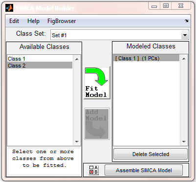
In order to build a SIMCA model, individual PCA models must be built on the data from each class (or group of classes). To build a PCA model:
- If multiple class sets are available in the data, select the class set to model using the "Class Set" control at the top of the window (Note: all models must use the same class set. Changing the class set during model building will clear all existing models.)
- Select one or more classes in the "Available Classes" list (Note: If more than one class is selected for an individual PCA model, these classes will be modeled as a single class.)
- Click "Fit Model" to activate the PCA user interface.
- In the PCA interface, validate and choose the appropriate number of components, preprocessing, etc.
- In the SIMCA interface click "Add Model".
- Repeat for additional models.
- Choose settings using the "SIMCA Model Options" button (A/B button next to Assemble SIMCA Model button)
- Click "Assemble SIMCA Model".
- Review the assembled SIMCA model using the main Analysis window.
- To classify new data, import new data into the Analysis interface and click "Prediction" to apply the assembled SIMCA model.
Below is an image of the SIMCA Model Building interface after one class model has been built.
Choosing the Classification Rule
Within the SIMCA Model Options is the classification "Rule". There are four options:
- Q
- T^2
- Both
- Combined
The following discusses each rule.
Q
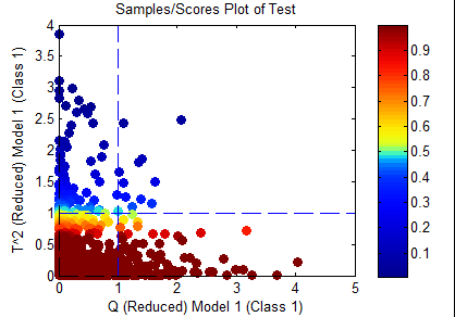
Only samples which are inside the Q confidence limit specified in the options will be considered "in-class". This would include only the samples in yellow and red in the figure below.
This option is one historically used by many researchers as the Q statistic is often very sensitive to differences between species.
T^2
Only samples which are inside the T^2 confidence limit specified in the options will be considered "in-class". This would include only the samples in yellow and red in the figure below.
This option is an unusual option as it is often the Q residuals which best separate classes. However, in a case where the Q may drift (due to instrumentation variations or noise), the T^2 could be more diagnostic of class differences.
Both
Only samples which are inside both the T^2 and Q confidence limits specified in the options will be considered "in-class". This would include only the samples in yellow and red in the figure below.
Although this option is somewhat intuitive, it does ignore the concept that the within-class variation of two separate classes are not necessarily orthogonal and, thus, the "combined" rule may be more sensitive (see below.)
Combined
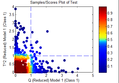
This rule first takes the Q and T^2 statistics "reduced" (normalized to) their confidence limits set in the options. Then the two statistics are combined using the equation:
Only samples inside the sqrt(2) limit will be considered "in-class". This would include only the samples in yellow and red in the figure below.
This option is quite useful because it allows differences in both T^2 and Q to be considered together. Although T^2 and Q are technically orthogonal statistics, the differences between classes are often not orthogonal but their class means are often different. Thus, a member of Class B would be expected to have both a projection into the model (indicated by the T^2) as well as residuals (indicated by the Q). Note that for a set of random data, this approach can be shown to reliably match the "true positive" rate expected for the given confidence limits.


