Model Building: Plotting Loads: Difference between revisions
imported>Jeremy No edit summary |
imported>Jeremy No edit summary |
||
| Line 6: | Line 6: | ||
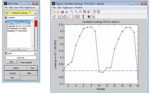
For most analysis methods, the Analysis window toolbar contains a Plot loads and variable statistics button [[Image:Plot_loads_variable_statistics_icon.png|21x20px]]. Loading is defined as the contribution of each variable to a principal component or factor. A Loads plot (also known as a Loadings plot) shows, at a minimum, as many different loadings as the number of principal components or factors that were retained in the model. Loads plots help you assess the extent to which the variables contribute to each of the individual principal components or factors. The figure below shows a Loads plots for a PCA analysis in which 20 variables were measured and three principal components were retained. In the Plot Controls window, three loadings-Loading on PC1, Loading on PC2, and Loading on PC3-are available for plotting. | For most analysis methods, the Analysis window toolbar contains a Plot loads and variable statistics button [[Image:Plot_loads_variable_statistics_icon.png|21x20px]]. Loading is defined as the contribution of each variable to a principal component or factor. A Loads plot (also known as a Loadings plot) shows, at a minimum, as many different loadings as the number of principal components or factors that were retained in the model. Loads plots help you assess the extent to which the variables contribute to each of the individual principal components or factors. The figure below shows a Loads plots for a PCA analysis in which 20 variables were measured and three principal components were retained. In the Plot Controls window, three loadings-Loading on PC1, Loading on PC2, and Loading on PC3-are available for plotting. | ||
:''Loads plots for a PCA analysis in which 20 variables were measured and three principal components were retained'' | |||
::[[Image:ModelBuilding_PlottingLoads.26.1.2.jpg|532x328px]] | ::[[Image:ModelBuilding_PlottingLoads.26.1.2.jpg|532x328px]] | ||
| Line 20: | Line 20: | ||
{| | {| | ||
|- | |- valign="top" | ||
| | | | ||
| Line 29: | Line 29: | ||
{| | {| | ||
|- | |- valign="top" | ||
| | | | ||
| Line 42: | Line 42: | ||
{| | {| | ||
|- | |- valign="top" | ||
| | | | ||
| Line 51: | Line 51: | ||
{| | {| | ||
|- | |- valign="top" | ||
| | | | ||
| Line 58: | Line 58: | ||
|} | |} | ||
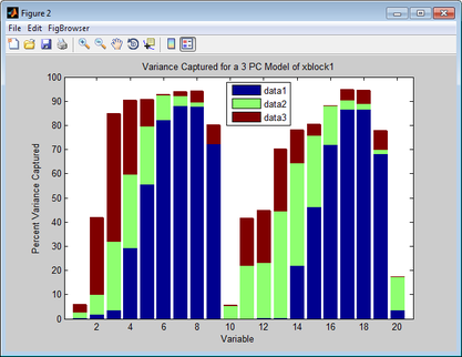
:''Example of a Variance Captured plot'' | |||
::[[Image:Varcap_plot.png|417x323px]] | ::[[Image:Varcap_plot.png|417x323px]] | ||
| Line 68: | Line 68: | ||
{| | {| | ||
|- | |- valign="top" | ||
| | | | ||
| Line 75: | Line 75: | ||
|} | |} | ||
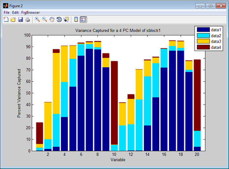
:''Example of a Variance Captured plot'' | |||
::[[Image:Varcap_plot_4pcs.png|466x345px]] | ::[[Image:Varcap_plot_4pcs.png|466x345px]] | ||
| Line 102: | Line 102: | ||
{| | {| | ||
|- | |- valign="top" | ||
|1. | |1. | ||
| Line 112: | Line 112: | ||
{| style="margin-left:18pt" | {| style="margin-left:18pt" | ||
|- | |- valign="top" | ||
| | | | ||
| Line 121: | Line 121: | ||
{| | {| | ||
|- | |- valign="top" | ||
|2. | |2. | ||
| Line 131: | Line 131: | ||
{| style="margin-left:18pt" | {| style="margin-left:18pt" | ||
|- | |- valign="top" | ||
| | | | ||
| Line 142: | Line 142: | ||
{| style="margin-left:18pt" | {| style="margin-left:18pt" | ||
|- | |- valign="top" | ||
| | | | ||
| Line 153: | Line 153: | ||
{| | {| | ||
|- | |- valign="top" | ||
|3. | |3. | ||
| Line 163: | Line 163: | ||
{| style="margin-left:18pt" | {| style="margin-left:18pt" | ||
|- | |- valign="top" | ||
| | | | ||
| Line 172: | Line 172: | ||
{| style="margin-left:18pt" | {| style="margin-left:18pt" | ||
|- | |- valign="top" | ||
| | | | ||
| Line 182: | Line 182: | ||
{| | {| | ||
|- | |- valign="top" | ||
| | | | ||
| Line 192: | Line 192: | ||
{| | {| | ||
|- | |- valign="top" | ||
| | | | ||
| Line 201: | Line 201: | ||
{| | {| | ||
|- | |- valign="top" | ||
|4. | |4. | ||
| Line 211: | Line 211: | ||
{| style="margin-left:18pt" | {| style="margin-left:18pt" | ||
|- | |- valign="top" | ||
| | | | ||
| Line 220: | Line 220: | ||
{| style="margin-left:18pt" | {| style="margin-left:18pt" | ||
|- | |- valign="top" | ||
| | | | ||
| Line 229: | Line 229: | ||
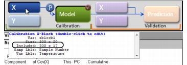
::Note: As shown in the figure below, after you exclude samples from a DataSet, point your mouse cursor on the X calibration control to open tooltip text opens that indicates the number of variables that are being included in the model. | ::Note: As shown in the figure below, after you exclude samples from a DataSet, point your mouse cursor on the X calibration control to open tooltip text opens that indicates the number of variables that are being included in the model. | ||
:''Tooltip text that indicates the number of variables that are being included in the model'' | |||
::[[Image:ModelBuilding_PlottingLoads.26.1.7.jpg|366x127px]] | ::[[Image:ModelBuilding_PlottingLoads.26.1.7.jpg|366x127px]] | ||
| Line 241: | Line 241: | ||
{| | {| | ||
|- | |- valign="top" | ||
| | | | ||
| Line 252: | Line 252: | ||
{| | {| | ||
|- | |- valign="top" | ||
| | | | ||
Revision as of 13:09, 29 July 2010
Table of Contents | Previous | Next
Plotting Loads and Variable Statistics for a Calibration Model
For most analysis methods, the Analysis window toolbar contains a Plot loads and variable statistics button ![]() . Loading is defined as the contribution of each variable to a principal component or factor. A Loads plot (also known as a Loadings plot) shows, at a minimum, as many different loadings as the number of principal components or factors that were retained in the model. Loads plots help you assess the extent to which the variables contribute to each of the individual principal components or factors. The figure below shows a Loads plots for a PCA analysis in which 20 variables were measured and three principal components were retained. In the Plot Controls window, three loadings-Loading on PC1, Loading on PC2, and Loading on PC3-are available for plotting.
. Loading is defined as the contribution of each variable to a principal component or factor. A Loads plot (also known as a Loadings plot) shows, at a minimum, as many different loadings as the number of principal components or factors that were retained in the model. Loads plots help you assess the extent to which the variables contribute to each of the individual principal components or factors. The figure below shows a Loads plots for a PCA analysis in which 20 variables were measured and three principal components were retained. In the Plot Controls window, three loadings-Loading on PC1, Loading on PC2, and Loading on PC3-are available for plotting.
- Loads plots for a PCA analysis in which 20 variables were measured and three principal components were retained
Note: For information about the Plot Controls window and Plot window, see Plot Controls Window.
Options are available for changing the plot display and for examining and refining the model by excluding certain samples and/or variables to enhance the model performance. See:
Changing the plot display
Note: The examples listed here are not meant to be an exhaustive list of all of the available Plot Controls options for changing a Loads plot display. Instead, it is simply to provide representative examples of some of the more commonly used options when building a model.
|
|
- Example of a Variance Captured plot
|
- Example of a Variance Captured plot
Refining the model by removing variables
Typically, when using Loads plots to refine a model, you select variables that you consider to be unusual for the plotted data and then carry out a series of steps to determine whether to include the variables in the model, or to exclude the variables from the model.
Note: Typically, if you want to refine a model by removing samples, you use the information in a Scores plot. See Plotting Scores and Statistical Values for a Calibration Model.
Note: The examples listed here are not meant to be an exhaustive list of all of the available Plot Controls options for refining a model using a Loads plot. Instead, it is simply to provide representative examples of some of the more commonly used options when building a model.
| 1. | Initially, you can do the following to review your variables, and determine which variables, if any, require further investigation: |
|
| 2. | For variables that you have determined require further investigation, you can do the following: |
- Note: "Lasso" is the most flexible tool for selecting samples.
- The color of the selected variable(s) is not only in the currently active plot, but also, in any other open plots that contain the variable(s).
| 3. | With the selected variables now highlighted in the plot, you can now do one or more of the following to place the focus on the selected variables and glean further information about the selected variables before deciding to include them or exclude them for the model: |
|
|
|
|
| 4. | To exclude all of the selected variables from the model in a single step, on the Plot Controls window main menu, click Edit > Exclude Selection. |
|
|
- Note: As shown in the figure below, after you exclude samples from a DataSet, point your mouse cursor on the X calibration control to open tooltip text opens that indicates the number of variables that are being included in the model.
- Tooltip text that indicates the number of variables that are being included in the model
At this point, you should iteratively repeat the steps of recalculating the model and then examining the model (in particular, by using the varcap plot) and refining the model by including or excluding variables until you are satisfied with the model. You can then do one of the following:
|
- Note: See Exporting_Models
|


