Bspcgui: Difference between revisions
imported>Scott No edit summary |
imported>Scott |
||
| (45 intermediate revisions by 3 users not shown) | |||
| Line 1: | Line 1: | ||
__TOC__ | __TOC__ | ||
=Introduction= | |||
Batch Statistical Process Control (BSPC) is the analysis of process data | Batch Statistical Process Control (BSPC) is the analysis of process data as a function of both correlation among the measured variables and correlation in time (also known as the batch trajectory). The data is subdivided into "batches" (experiments) each of which may be further subdivided into "Steps" (sub-divisions of batch indicating processing segments or other divisions of batches). BSPC goes by many names, process monitoring, fault detection, and anomaly detection, to name a few. Methods generally rely on a model that describes normal and/or desirable operation. Often much is learned about the process from simply the creation of a model. Given a process model, future operating data can be compared to the model to determine if the process condition is nominal. | ||
The BSPC interface is available in Solo or the PLS_Toolbox browser window in the "Analysis Tools" panel under the "TRANSFORM" label as "Batch Processor". This interface prompts the user to select a type of analysis method they want to do, then guides the user through the steps necessary to use that method including: | |||
# Importing and organizing the batch data | |||
# Assuring the batch and step labels (if desired) are assigned | |||
# Aligning the time axes of the batches (if needed for the specific analysis method) | |||
# Choosing other data manipulation settings as needed for the method | |||
# Rearranging the data to the appropriate format for the specific analysis method using the [[batchfold]] function | |||
=Getting Started= | |||
Data is derived directly from process data with the goal being to summarize high-dimensional data with a handful of factors that capture important directions in the data. Success is highly dependent upon the quantity and quality of process data. | |||
Raw data is presumed to be in a 2 dimensional DataSet with rows being samples in time and columns being variables. | |||
[[Image:bspc_data_config.png|200px|Data Configuration]] | |||
===Model Types=== | ===Model Types=== | ||
The following describes the model types available as targets of the BSPC processing. The dimensions of the resulting processed data and other considerations are listed along with a brief description of the unique characteristics of the model type. | |||
{| class="wikitable" border="1" | {| class="wikitable" border="1" | ||
|+ BSPC Model Types | |+ BSPC Model Types | ||
! Model !! Modes (Dimensions) !! Equal Length Batches !! Steps Aligned !! Comments | ! Model !! Modes (Dimensions) !! Equal Length Batches !! Steps Aligned !! Data Shape !! Model Comments | ||
|- | |- | ||
| Summary PCA || 2 || No || No || | | Summary PCA || 2 || No || No || Batch x (Step/Summary) || PCA on statistics summarizing the change in measured variables over the batch progress. Less sensitive to specific batch trajectory. | ||
|- | |- | ||
| Batch Maturity || 2 || No || No || Can have Y-Block to indicate maturity | | [[Batchmaturity|Batch Maturity]] || 2 || No || No || (Batch/Step) x Variable, Can have Y-Block to indicate maturity || PCA with heterogeneous confidence limits based on percent progression through batch. | ||
|- | |- | ||
| MPCA || 3 || Yes || Yes || | | [[Mpca|MPCA]] || 3 || Yes || Yes || Time (step) x Variable x Batch || Multiway PCA - captures correlation between variables and their changes through time (trajectory). Very sensitive to trajectory differences. | ||
|- | |- | ||
| PARAFAC || 3 || Yes || Yes || | | [[Parafac|PARAFAC]] || 3 || Yes || Yes || Batch x Variable x Time (step) || Parallel Factor Analysis (multiway). Imposes stronger expectation of similarity between variable trajectories than MPCA. | ||
|- | |- | ||
| Summary PARAFAC || 3 || No || No || | | Summary PARAFAC || 3 || No || No || Batch x Step x Summary || PARAFAC on summary statistics of variables over time. Less sensitive to specific batch trajectory, imposes expectation of correlation between steps of process. | ||
|- | |- | ||
| PARAFAC2 || 3 || No || No || | | [[Parafac2|PARAFAC2]] || 3 || No || No || Cell Array of Batches || PARAFAC with relaxed multiway structures (only available at PLS_Toolbox command line). Much less sensitive to specific batch trajectory than PARAFAC or MPCA. | ||
|} | |} | ||
See Also: [[batchmaturity|Batch Maturity]], [[mpca|MPCA]], [[MSPC_and_Identification_of_Finite_Impulse_Response_Models|MSPC]], [[parafac|PARAFAC]], [[parafac2|PARAFAC2]] | |||
The goal of the Batch Processor interface is to make it easier to assemble | =Batch Processor Window= | ||
The goal of the Batch Processor interface is to make it easier to assemble batch data for multivariate analysis. Different analyses and conditions require different data manipulation. This interface attempts to simplify the assembling of data for batch analysis which might otherwise be [[media:Bspc_diagram_roadmap.png | very complicated]]. | |||
The workflow of the interface moves from left to right across the tabs at the top of the interface. Loading data and choosing an Analysis Type will enable relevant tabs. Clicking the '''Next''' button will open the next enabled tab. Batches and steps are defined, then alignment and summary information is added. When finished, "folded" data can be saved or exported to the [[Analysis GUI|analysis]] interface and a model for folding new data can be saved. | |||
[[Image:BSPCGUI main.png| BSPC GUI]] | [[Image:BSPCGUI main.png| BSPC GUI]] | ||
==Start== | |||
Load, append, edit, and or clear data. Selecting the Analysis type will automatically enable/disable relevant tabs. | Load, append, edit, and or clear data. Selecting the Analysis type will automatically enable/disable relevant tabs. | ||
* Dropping data onto the status area will load data. If previously loaded exists, a prompt for overwrite or augment will appear. | * Dropping data onto the status area will load data. If previously loaded data exists, a prompt for overwrite or augment will appear. | ||
** If augment is chosen, two options will be given, augment as new batch or not. Augment as new batch adds a class for the data being augmented otherwise a "normal" augment will occur and if the new dataset has a matching class it will be merged. | ** If augment is chosen, two options will be given, augment as new batch or not. Augment as new batch adds a class for the data being augmented otherwise a "normal" augment will occur and if the new dataset has a matching class it will be merged. | ||
* Dragging and dropping multiple-selected (Excel) files from the system | * Dragging and dropping multiple-selected (Excel) files from the system browser (e.g., Windows Explorer or Finder) will pre-augment the files and create a label indicating file name. This label can be used to identify batches in the '''Batches''' tab. | ||
* Data can be edited in the [[DataSet Editor]] by clicking the '''Edit''' button. Editing will cause the model to be cleared. | * Data can be edited in the [[DataSet Editor]] by clicking the '''Edit''' button. Editing will cause the model to be cleared. | ||
==Batch== | |||
Indicates which samples belong to which batch based on information in the loaded DataSet. Sources can be Class, Label, or Axisscale sets, or a single Variable (column). If manually loaded, a class is created from the loaded content. If the DataSet contains a class with the default name of "BSPC Batch" then it will be automatically selected after loading. | |||
* If variable is used, data for that column will be excluded (not deleted) so other mechanisms (preprocessing) can work. | * If variable is used, data for that column will be excluded (not deleted) so other mechanisms (preprocessing) can work. | ||
* Once Batches have been identified, one or more batches can be plotted in the lower plot. | |||
All methods, except [[batchmaturity|Batch Maturity]] require defining a means to identify the different batches because these are used to form the samples of the input matrices (and multiple samples are required for all methods other than Batch Maturity). | |||
==Steps== | |||
Steps (subdivisions of batches) can be indicated on the '''Steps''' tab. Steps can be created in the same manor as '''Batches''' or indicated manually. Particular steps to be included or excluded can be selected. | |||
Manual selection is done by selecting a primary variable and batch to align '''to''' then designating '''steps''' for the primary variable/batch. After the steps are set the [[batchalign]] function is used to "map" step location (as dataset class) for each batch. | |||
===Manually Selecting Steps=== | |||
[[Image:bspc_manual_select.png|500px|Manual Selection Interface]] | |||
To manually select steps: | |||
# Select the variable and batch to use from the plot list boxes at the bottom of the interface. These will become the variable and batch to which all others are aligned to (designated by a "*" next to the list item. | |||
# Click the '''Select''' button and the interface will switch. | |||
# Click the '''Add''' button to place the first step marker. | |||
# Drag this marker to the first step location. | |||
# Repeat until all steps are placed. | |||
# Select different batch from list menu to display "aligned" step position. | |||
# Adjust alignment algorithm as needed using toolbar button. | |||
# Click check-mark button to finish and save steps. | |||
===Selected Steps Menu=== | |||
[[Image:bspc_selected_steps.png|300px|]] | |||
Once steps have been designated, they will appear the '''Step Selection''' list. If one or more steps should be ignored they can be deselected in this menu. Selected steps will appear in the batch plot as solid green lines and unselected steps appear as red dashed lines. | |||
==Align== | |||
Methods that require equal length batches use the tools available on the '''Align''' tab from the [[batchalign]] function. | |||
The process to configure the alignment is: | |||
# Select the type of alignment: | |||
#* '''Linear''' - Linear interpolation or decimation to match selected batch's length. | |||
#* '''COW''' - [[cow|Correlation Optimized Warping]] with Alignment Settings values. | |||
#* '''Pad With NaN''' - Append each batch with NaN to make all batches equal length. | |||
# Select the Batch and Variable to use as a reference (target) or Load a vector. | |||
# Select alignment settings (if using COW). | |||
# Click Update Plot to see the results. | |||
The plots switch to displaying selected variables and batches with the pre-aligned data on top and post-aligned data on the bottom. Click the '''Update Plots''' button to refresh the plot after making any changes. | |||
[[Image:bspc_align_settings.png|Align Settings ]] | |||
NOTE: In the image above, the alignment batch is Class 0 (the default) which has no members. This must be changed before alignment will work. | |||
==Summarize== | |||
The summary PCA and summary PARAFAC methods make use of statistical summary functions to capture the trends in the trajectories of the variables. A Summary PCA or Summary PARAFAC model does not require alignment of batches and is generally less sensitive to the exact trajectory of the batches, providing some model robustness. | |||
The statistics are calculated by the [[summary]] function and have different sensitivities to profile changes. The ability of each statistic to capture useful information from a trajectory depends on the dynamics and the statistic. Often it is useful to include a number of the statistics and decide, while modeling, which seem to be providing information and excluding the remaining statistics. If the statistics are sufficiently sensitive to the trajectory profile as to provide detection of out-of-specification batches, then the model will likely provide longer-term performance over an equivalent MPCA or PARAFAC model. | |||
The statistics which are available include: | |||
[[Image:Bspc_summarize.png|Summary Options]] | |||
All stats summarize each column and each step (if specified) except for: | |||
* '''Length''' Length of step = a single number for each step (irrespective of number of variables). | |||
* '''Five-Number Summary''' 10, 25, 50, 75, 90th percentile = 5 values per step per variable. | |||
For example with the [[Demonstration_Datasets | Dupont]] demo calibration data (dupont_cal), if you choose mean, std, slope, skewness, and length the size of your folded summary pca data will be: | |||
10 variables x 4 stats + length = 41 values per step * 5 steps = 205 columns | |||
==Finish== | |||
When completed there are 4 options: | |||
* Send data directly to a new [[Analysis]] window. | |||
* Save the data to the workspace. | |||
* Save a model for future data application. NOTE: In some more complicated instances (loading outside information) the model may not be able to fully capture each step taken in the interface. | |||
* Cancel and close the window. | |||
Latest revision as of 10:21, 6 September 2017
Introduction
Batch Statistical Process Control (BSPC) is the analysis of process data as a function of both correlation among the measured variables and correlation in time (also known as the batch trajectory). The data is subdivided into "batches" (experiments) each of which may be further subdivided into "Steps" (sub-divisions of batch indicating processing segments or other divisions of batches). BSPC goes by many names, process monitoring, fault detection, and anomaly detection, to name a few. Methods generally rely on a model that describes normal and/or desirable operation. Often much is learned about the process from simply the creation of a model. Given a process model, future operating data can be compared to the model to determine if the process condition is nominal.
The BSPC interface is available in Solo or the PLS_Toolbox browser window in the "Analysis Tools" panel under the "TRANSFORM" label as "Batch Processor". This interface prompts the user to select a type of analysis method they want to do, then guides the user through the steps necessary to use that method including:
- Importing and organizing the batch data
- Assuring the batch and step labels (if desired) are assigned
- Aligning the time axes of the batches (if needed for the specific analysis method)
- Choosing other data manipulation settings as needed for the method
- Rearranging the data to the appropriate format for the specific analysis method using the batchfold function
Getting Started
Data is derived directly from process data with the goal being to summarize high-dimensional data with a handful of factors that capture important directions in the data. Success is highly dependent upon the quantity and quality of process data.
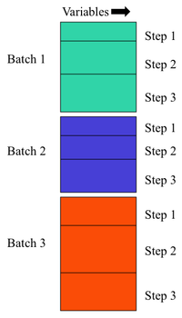
Raw data is presumed to be in a 2 dimensional DataSet with rows being samples in time and columns being variables.
Model Types
The following describes the model types available as targets of the BSPC processing. The dimensions of the resulting processed data and other considerations are listed along with a brief description of the unique characteristics of the model type.
| Model | Modes (Dimensions) | Equal Length Batches | Steps Aligned | Data Shape | Model Comments |
|---|---|---|---|---|---|
| Summary PCA | 2 | No | No | Batch x (Step/Summary) | PCA on statistics summarizing the change in measured variables over the batch progress. Less sensitive to specific batch trajectory. |
| Batch Maturity | 2 | No | No | (Batch/Step) x Variable, Can have Y-Block to indicate maturity | PCA with heterogeneous confidence limits based on percent progression through batch. |
| MPCA | 3 | Yes | Yes | Time (step) x Variable x Batch | Multiway PCA - captures correlation between variables and their changes through time (trajectory). Very sensitive to trajectory differences. |
| PARAFAC | 3 | Yes | Yes | Batch x Variable x Time (step) | Parallel Factor Analysis (multiway). Imposes stronger expectation of similarity between variable trajectories than MPCA. |
| Summary PARAFAC | 3 | No | No | Batch x Step x Summary | PARAFAC on summary statistics of variables over time. Less sensitive to specific batch trajectory, imposes expectation of correlation between steps of process. |
| PARAFAC2 | 3 | No | No | Cell Array of Batches | PARAFAC with relaxed multiway structures (only available at PLS_Toolbox command line). Much less sensitive to specific batch trajectory than PARAFAC or MPCA. |
See Also: Batch Maturity, MPCA, MSPC, PARAFAC, PARAFAC2
Batch Processor Window
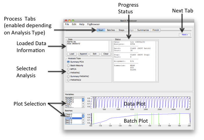
The goal of the Batch Processor interface is to make it easier to assemble batch data for multivariate analysis. Different analyses and conditions require different data manipulation. This interface attempts to simplify the assembling of data for batch analysis which might otherwise be very complicated.
The workflow of the interface moves from left to right across the tabs at the top of the interface. Loading data and choosing an Analysis Type will enable relevant tabs. Clicking the Next button will open the next enabled tab. Batches and steps are defined, then alignment and summary information is added. When finished, "folded" data can be saved or exported to the analysis interface and a model for folding new data can be saved.
Start
Load, append, edit, and or clear data. Selecting the Analysis type will automatically enable/disable relevant tabs.
- Dropping data onto the status area will load data. If previously loaded data exists, a prompt for overwrite or augment will appear.
- If augment is chosen, two options will be given, augment as new batch or not. Augment as new batch adds a class for the data being augmented otherwise a "normal" augment will occur and if the new dataset has a matching class it will be merged.
- Dragging and dropping multiple-selected (Excel) files from the system browser (e.g., Windows Explorer or Finder) will pre-augment the files and create a label indicating file name. This label can be used to identify batches in the Batches tab.
- Data can be edited in the DataSet Editor by clicking the Edit button. Editing will cause the model to be cleared.
Batch
Indicates which samples belong to which batch based on information in the loaded DataSet. Sources can be Class, Label, or Axisscale sets, or a single Variable (column). If manually loaded, a class is created from the loaded content. If the DataSet contains a class with the default name of "BSPC Batch" then it will be automatically selected after loading.
- If variable is used, data for that column will be excluded (not deleted) so other mechanisms (preprocessing) can work.
- Once Batches have been identified, one or more batches can be plotted in the lower plot.
All methods, except Batch Maturity require defining a means to identify the different batches because these are used to form the samples of the input matrices (and multiple samples are required for all methods other than Batch Maturity).
Steps
Steps (subdivisions of batches) can be indicated on the Steps tab. Steps can be created in the same manor as Batches or indicated manually. Particular steps to be included or excluded can be selected.
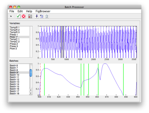
Manual selection is done by selecting a primary variable and batch to align to then designating steps for the primary variable/batch. After the steps are set the batchalign function is used to "map" step location (as dataset class) for each batch.
Manually Selecting Steps
To manually select steps:
- Select the variable and batch to use from the plot list boxes at the bottom of the interface. These will become the variable and batch to which all others are aligned to (designated by a "*" next to the list item.
- Click the Select button and the interface will switch.
- Click the Add button to place the first step marker.
- Drag this marker to the first step location.
- Repeat until all steps are placed.
- Select different batch from list menu to display "aligned" step position.
- Adjust alignment algorithm as needed using toolbar button.
- Click check-mark button to finish and save steps.
Selected Steps Menu
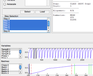
Once steps have been designated, they will appear the Step Selection list. If one or more steps should be ignored they can be deselected in this menu. Selected steps will appear in the batch plot as solid green lines and unselected steps appear as red dashed lines.
Align
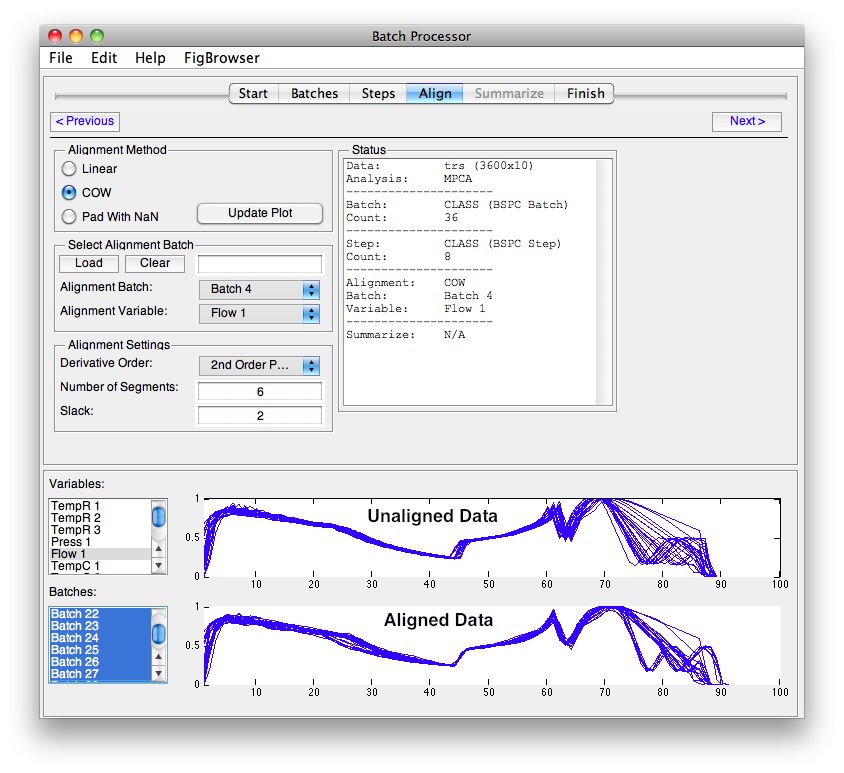
Methods that require equal length batches use the tools available on the Align tab from the batchalign function.
The process to configure the alignment is:
- Select the type of alignment:
- Linear - Linear interpolation or decimation to match selected batch's length.
- COW - Correlation Optimized Warping with Alignment Settings values.
- Pad With NaN - Append each batch with NaN to make all batches equal length.
- Select the Batch and Variable to use as a reference (target) or Load a vector.
- Select alignment settings (if using COW).
- Click Update Plot to see the results.
The plots switch to displaying selected variables and batches with the pre-aligned data on top and post-aligned data on the bottom. Click the Update Plots button to refresh the plot after making any changes.
NOTE: In the image above, the alignment batch is Class 0 (the default) which has no members. This must be changed before alignment will work.
Summarize
The summary PCA and summary PARAFAC methods make use of statistical summary functions to capture the trends in the trajectories of the variables. A Summary PCA or Summary PARAFAC model does not require alignment of batches and is generally less sensitive to the exact trajectory of the batches, providing some model robustness.
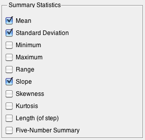
The statistics are calculated by the summary function and have different sensitivities to profile changes. The ability of each statistic to capture useful information from a trajectory depends on the dynamics and the statistic. Often it is useful to include a number of the statistics and decide, while modeling, which seem to be providing information and excluding the remaining statistics. If the statistics are sufficiently sensitive to the trajectory profile as to provide detection of out-of-specification batches, then the model will likely provide longer-term performance over an equivalent MPCA or PARAFAC model.
The statistics which are available include:
All stats summarize each column and each step (if specified) except for:
- Length Length of step = a single number for each step (irrespective of number of variables).
- Five-Number Summary 10, 25, 50, 75, 90th percentile = 5 values per step per variable.
For example with the Dupont demo calibration data (dupont_cal), if you choose mean, std, slope, skewness, and length the size of your folded summary pca data will be:
10 variables x 4 stats + length = 41 values per step * 5 steps = 205 columns
Finish
When completed there are 4 options:
- Send data directly to a new Analysis window.
- Save the data to the workspace.
- Save a model for future data application. NOTE: In some more complicated instances (loading outside information) the model may not be able to fully capture each step taken in the interface.
- Cancel and close the window.
