SpectraQuant Filtering: Difference between revisions
imported>Jeremy |
imported>Donal No edit summary |
||
| (10 intermediate revisions by one other user not shown) | |||
| Line 1: | Line 1: | ||
__TOC__ | __TOC__ | ||
SpectraQuant Filtering is a preprocessing method used to remove interferences from data prior to building a regression model. The SpectraQuant filter includes one or more of the following corrections: | |||
# multivariate filtering of components defined by a set of clutter or "correction" spectra. | # multivariate filtering of components defined by a set of clutter or "correction" spectra. | ||
| Line 6: | Line 6: | ||
# an integrated thickness/pathlength correction. | # an integrated thickness/pathlength correction. | ||
== | ==SpectraQuant Filtering Panel== | ||
The | The SpectraQuant Filtering tools are accessed through the SpectraQuant Filtering panel of Analysis GUI (click on the "Filter Settings" button just below the top status panel). The filter settings panel is only available when using the PCR or PLS Analysis methods and only enabled when calibration data has already been loaded. The default settings for the panel are shown below. | ||
[[Image:Cpsa_panel_empty.png]] | [[Image:Cpsa_panel_empty.png]] | ||
| Line 15: | Line 15: | ||
Four different options categories are available on the panel: | Four different options categories are available on the panel: | ||
* '''[[ | * '''[[SpectraQuant_Filtering#Correction_Spectra | Correction Spectra]]''' - Allows selecting correction spectra which describe background components which should be removed from the spectra prior to analysis. | ||
* '''[[ | * '''[[SpectraQuant_Filtering#Regions.2FBaselines | Regions/Baselines]]''' - Defines regions of the spectra and the baseline order to apply to each region. | ||
* '''[[ | * '''[[SpectraQuant_Filtering#Thickness_Correction | Thickness Correction]]''' - Determines whether or not to use thickness/pathlength correction (requires thickness/pathlength reference in calibration data) | ||
* '''[[ | * '''[[SpectraQuant_Filtering#Force_PC80_Compatible_Preprocessing | Force PC80 Compatible Preprocessing]]''' - Determines whether to enforce strict preprocessing rules on the created model. | ||
==Correction Spectra== | ==Correction Spectra== | ||
| Line 31: | Line 31: | ||
===Adding Correction Spectra=== | ===Adding Correction Spectra=== | ||
To add correction spectra to the filter, click on the '''Add''' button and select the file type to read (e.g. " | To add correction spectra to the filter, click on the '''Add''' button and select the file type to read (e.g. "AIT ASF files") and click OK. | ||
Browse to the folder containing the file(s) to load, select one or more files (using shift-click or control-click to select multiple files), and click "Open". | Browse to the folder containing the file(s) to load, select one or more files (using shift-click or control-click to select multiple files), and click "Open". | ||
| Line 45: | Line 45: | ||
===Choosing Number of Factors=== | ===Choosing Number of Factors=== | ||
The | The SpectraQuant filter calculates a PCA model from the correction spectra and keeps some number of factors. The edit box on the right of the control specifies the number of factors to use in the filter. The higher the number, the more degrees of freedom the filter will remove (and the increased chance of removing useful signal). In general, a lower number of factors is recommended unless the filter is not performing sufficiently for a given application. | ||
===Viewing the Correction Spectra=== | ===Viewing the Correction Spectra=== | ||
| Line 53: | Line 53: | ||
==Regions/Baselines== | ==Regions/Baselines== | ||
By default, all spectral regions marked as "included" in the X-block data will be used in the calibration model. However, the Regions/Baselines option of the | By default, all spectral regions marked as "included" in the X-block data will be used in the calibration model. However, the Regions/Baselines option of the filter settings panel allows selection of specific spectral sub-regions to include (and, conversely, to discard other regions). In addition, the selected sub-regions can be detrended (i.e. baselined across the entire selected region). | ||
To select one or more specific sub-regions, click the '''Edit''' button next to the Regions/Baselines option on the | To select one or more specific sub-regions, click the '''Edit''' button next to the Regions/Baselines option on the filter settings panel. This will bring up the Regions and Baselines GUI. Initially, no regions will be selected and you will see the mean of all the calibration spectra and an empty table at the bottom of the GUI (see figure below.) Note that all changes within the Regions and Baselines GUI take effect immediately. | ||
If you want to view a specific spectrum or spectra in the calibration data instead of the mean, select the Plot/Rows menu item in the Plot Controls, then select the spectrum/spectra to view in the Plot Controls. | If you want to view a specific spectrum or spectra in the calibration data instead of the mean, select the Plot/Rows menu item in the Plot Controls, then select the spectrum/spectra to view in the Plot Controls. | ||
| Line 79: | Line 79: | ||
Once created, regions can be edited by either directly editing the values in the table, or by clicking and dragging the dark region markers on the left and right edges of each region in the plot. | Once created, regions can be edited by either directly editing the values in the table, or by clicking and dragging the dark region markers on the left and right edges of each region in the plot. | ||
In addition to specifying the included spectral range, the table also allows specifying the order of polynomial to use | In addition to specifying the included spectral range, the table also allows specifying the order of baseline polynomial to use and the grouping of regions (Note that although the terminology here is "baseline", the calculation is, in fact, a "detrend" in which the polynomial is fit to the entire range of windowed intensities.) | ||
In the example above, the specified window will be baselined using a 2nd order (Quadratic) polynomial. | Grouping of regions requires that separate regions be fit with a single set of baseline polynomials. Normally, each region's baseline is fit independently. When regions are grouped, a single set of polynomial functions is simultaneously fit to all regions in the group. Note that all regions in a group will be forced to use the same polynomial order. To group two or more regions, simply change the "group #" for each region to the same value. Regions will automatically be colored the same (to indicate they are grouped) and the polynomial orders "linked". | ||
Grouping regions effectively allows the creation of a "gap" around an unwanted feature in a single region because two regions which span the unwanted feature can be grouped making them act as one. | |||
In the example above, the specified window will be baselined using a 2nd order (Quadratic) polynomial. Since there is only one region, no grouping can be done. | |||
===Removing Regions=== | ===Removing Regions=== | ||
To remove a region, either select the corresponding row in the table at the bottom of the GUI and press the [-] toolbar button, or right-click the region and select '''Remove Region''' from the context menu. In the example below, the | To remove a region, either select the corresponding row in the table at the bottom of the GUI and press the [-] toolbar button, or right-click the region and select '''Remove Region''' from the context menu. In the example below, the green region has been right-clicked giving the Remove Region context menu. | ||
[[Image:Cpsa_regions_delete.png]] | [[Image:Cpsa_regions_delete.png]] | ||
| Line 101: | Line 105: | ||
==Force PC80 Compatible Preprocessing== | ==Force PC80 Compatible Preprocessing== | ||
If this option is unchecked, the user may use any preprocessing available in the custom | If this option is unchecked, the user may use any preprocessing available in the custom preprocessing interface. The model created will be compatible with Eigenvector Research software such as Solo_Predictor, Solo, and PLS_Toolbox but may not be compatible with the AIT PC80 and CPSA32 applications. | ||
When checked, the preprocessing selected in the pull-down menu to the right of the option (including: None, Mean Centering, Autoscaling) will be used and any other preprocessing manually selected from the Custom preprocessing GUI or the preprocessing menus will be removed. This mode assures that the model created will be as compatible as possible with the PC80 and CPSA32 applications. | When checked, the preprocessing selected in the pull-down menu to the right of the option (including: None, Mean Centering, Autoscaling) will be used and any other preprocessing manually selected from the Custom preprocessing GUI or the preprocessing menus will be removed. This mode assures that the model created will be as compatible as possible with the PC80 and CPSA32 applications. | ||
Latest revision as of 10:36, 26 April 2012
SpectraQuant Filtering is a preprocessing method used to remove interferences from data prior to building a regression model. The SpectraQuant filter includes one or more of the following corrections:
- multivariate filtering of components defined by a set of clutter or "correction" spectra.
- detrending (aka baselining) of the input data in windows of variables.
- an integrated thickness/pathlength correction.
SpectraQuant Filtering Panel
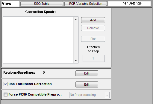
The SpectraQuant Filtering tools are accessed through the SpectraQuant Filtering panel of Analysis GUI (click on the "Filter Settings" button just below the top status panel). The filter settings panel is only available when using the PCR or PLS Analysis methods and only enabled when calibration data has already been loaded. The default settings for the panel are shown below.
Four different options categories are available on the panel:
- Correction Spectra - Allows selecting correction spectra which describe background components which should be removed from the spectra prior to analysis.
- Regions/Baselines - Defines regions of the spectra and the baseline order to apply to each region.
- Thickness Correction - Determines whether or not to use thickness/pathlength correction (requires thickness/pathlength reference in calibration data)
- Force PC80 Compatible Preprocessing - Determines whether to enforce strict preprocessing rules on the created model.
Correction Spectra
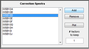
The list on the left of this option shows the file(s) which have been selected by the user as correction spectra (aka background or clutter spectra) which should be removed from all calibration and test spectra. To perform the filter, the correction spectra are first decomposed using a Principal Component Analysis (PCA) model containing a user-specified number of principal components or "factors". The resulting factors are then used as the filter.
If no correction spectra are loaded, no background removal will occur, but all other filter steps (see other options) will still be completed.
Adding Correction Spectra
To add correction spectra to the filter, click on the Add button and select the file type to read (e.g. "AIT ASF files") and click OK.
Browse to the folder containing the file(s) to load, select one or more files (using shift-click or control-click to select multiple files), and click "Open".
The files will be loaded and added to the list. You will be advised if the spectral axis of the loaded files appears to be incompatible with the currently loaded x-block data. Any incompatible spectra will not be loaded.
Removing Correction Spectra
Any file that has been loaded as a correction spectrum can be removed from the filter by simply clicking on the filename in the list on the left, and then clicking on the Remove button. The file will be discarded. Note that after discarding any spectra from the filter, any currently-loaded model will be cleared and have to be recalculated because the filter has now changed and the model is no longer current.
Choosing Number of Factors
The SpectraQuant filter calculates a PCA model from the correction spectra and keeps some number of factors. The edit box on the right of the control specifies the number of factors to use in the filter. The higher the number, the more degrees of freedom the filter will remove (and the increased chance of removing useful signal). In general, a lower number of factors is recommended unless the filter is not performing sufficiently for a given application.
Viewing the Correction Spectra
The selected correction spectra can be viewed in a plot by clicking the Plot button. The spectra selected on the left will be displayed, but all loaded correction spectra can be viewed using the Plot Controls which will appear along with the plot of the spectra. Regions of these spectra can be excluded using the Select button and Edit/Exclude or Include menu options in the Plot Controls.
Regions/Baselines
By default, all spectral regions marked as "included" in the X-block data will be used in the calibration model. However, the Regions/Baselines option of the filter settings panel allows selection of specific spectral sub-regions to include (and, conversely, to discard other regions). In addition, the selected sub-regions can be detrended (i.e. baselined across the entire selected region).
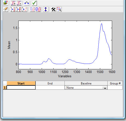
To select one or more specific sub-regions, click the Edit button next to the Regions/Baselines option on the filter settings panel. This will bring up the Regions and Baselines GUI. Initially, no regions will be selected and you will see the mean of all the calibration spectra and an empty table at the bottom of the GUI (see figure below.) Note that all changes within the Regions and Baselines GUI take effect immediately.
If you want to view a specific spectrum or spectra in the calibration data instead of the mean, select the Plot/Rows menu item in the Plot Controls, then select the spectrum/spectra to view in the Plot Controls.
The toolbar on this figure provides several options:
- Folder Icon - import regions and baselines from a CPSA32 .cri file
- [+] Icon - add a new region (click and drag)
- [-] Icon - remove the region currently selected in the table at the bottom of the GUI
- Double-arrow Icon - reverse the x-axis direction
- Check Mark Icon - accept the current regions and close the GUI
Adding Regions and Baselines
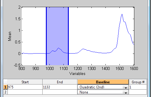
To begin selecting regions, either enter the starting and ending frequencies in an empty line in the table at the bottom of the GUI or click the [+] toolbar button and click-and-drag a new region on the interface. In the figure below, the user has manually entered a starting and ending value creating the first region (shown as shaded blue region in the plot.)
Once created, regions can be edited by either directly editing the values in the table, or by clicking and dragging the dark region markers on the left and right edges of each region in the plot.
In addition to specifying the included spectral range, the table also allows specifying the order of baseline polynomial to use and the grouping of regions (Note that although the terminology here is "baseline", the calculation is, in fact, a "detrend" in which the polynomial is fit to the entire range of windowed intensities.)
Grouping of regions requires that separate regions be fit with a single set of baseline polynomials. Normally, each region's baseline is fit independently. When regions are grouped, a single set of polynomial functions is simultaneously fit to all regions in the group. Note that all regions in a group will be forced to use the same polynomial order. To group two or more regions, simply change the "group #" for each region to the same value. Regions will automatically be colored the same (to indicate they are grouped) and the polynomial orders "linked".
Grouping regions effectively allows the creation of a "gap" around an unwanted feature in a single region because two regions which span the unwanted feature can be grouped making them act as one.
In the example above, the specified window will be baselined using a 2nd order (Quadratic) polynomial. Since there is only one region, no grouping can be done.
Removing Regions
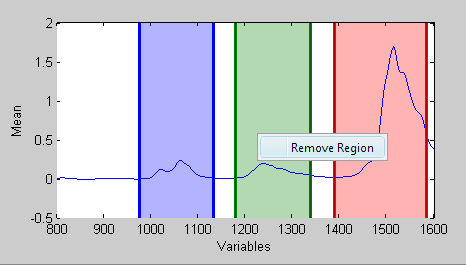
To remove a region, either select the corresponding row in the table at the bottom of the GUI and press the [-] toolbar button, or right-click the region and select Remove Region from the context menu. In the example below, the green region has been right-clicked giving the Remove Region context menu.
Thickness Correction
The thickness / pathlength correction option allows automatic detection and correction of pathlength errors. To make this correction, the calibration data must be loaded with pathlength values in the sample axisscale of the X-block (note that the name of the axisscale must be "pathlength"). The values supplied will be used to calculate a correction model which, when applied to future data, will attempt to correct any pathlength variations detected in that data.
To enable this feature, check the Use Thickness Correction checkbox. If no pathlength data was supplied with the calibration X-block spectra, you will be prompted to specify a default value to assign to all spectra. These default values, or any values supplied when importing the spectra, can be modified by clicking the Edit button to the right of this option.
Editing the pathlength will open a DataSet editor for the X-block with the Row Labels tab selected. The Axis Scale column of this interface contains the pathlength values. These values can be manually corrected, or copied and/or pasted from another application. To copy the current values or paste in new values, click on the Axis Scale button at the top of the interface, then select the menu: Edit/Copy or Edit/Paste. All changes in the DataSet editor take effect immediately.
Uncheck the Use Thickness Correction checkbox to disable the thickness correction feature.
Force PC80 Compatible Preprocessing
If this option is unchecked, the user may use any preprocessing available in the custom preprocessing interface. The model created will be compatible with Eigenvector Research software such as Solo_Predictor, Solo, and PLS_Toolbox but may not be compatible with the AIT PC80 and CPSA32 applications.
When checked, the preprocessing selected in the pull-down menu to the right of the option (including: None, Mean Centering, Autoscaling) will be used and any other preprocessing manually selected from the Custom preprocessing GUI or the preprocessing menus will be removed. This mode assures that the model created will be as compatible as possible with the PC80 and CPSA32 applications.
