Declutter Settings Window: Difference between revisions
imported>Jeremy m (moved GLSW Settings GUI to Declutter Settings Window) |
No edit summary |
||
| (18 intermediate revisions by 3 users not shown) | |||
| Line 1: | Line 1: | ||
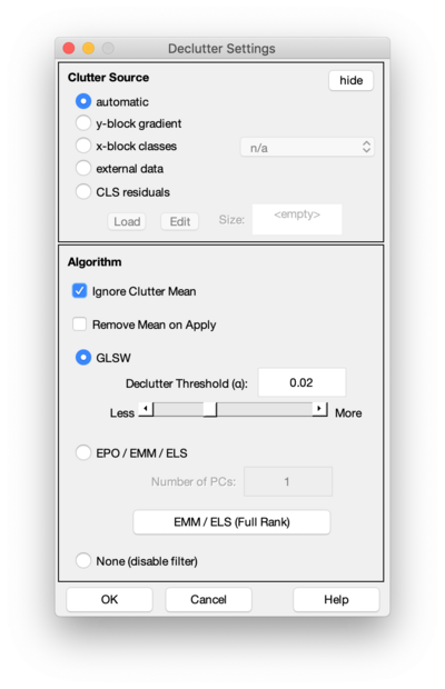
The '''Declutter Settings window''' allows modification of the settings for the Generalized Least Squares Weighting (GLSW), External Parameter Orthgonalization (EPO), and Extended Mixture Model (EMM) filters. | |||
GLSW, EPO, and EMM are [[Advanced_Preprocessing:_Multivariate_Filtering|"multivariate filters"]] which identify patterns in the variables of the data which should be down-weighted or removed. Multivariate filters (a.k.a. "covariance filters") are an effective way to remove interfering signal (known as "clutter") from data prior to building a model. This page describes the different options controlled by the settings window. The uses of these filters and the algorithmic details can be found on the [[Advanced_Preprocessing:_Multivariate_Filtering|Advanced Preprocessing: Multivariate Filtering]] page and also on the [[glsw|the glsw function help page]]. | |||
[[File:Declutter_gui_1.png | 400px ]] | |||
===Clutter Source=== | ===Clutter Source=== | ||
| Line 10: | Line 10: | ||
* '''x-block classes''': Used when the data contains classes which define sets of "similar" samples. The filter will down-weight features which make the data diverse within each class. The first class set defined for the x-block rows (samples) will be used to group samples. Class zero will be ignored, but all other classes will be combined and the differences within each class will be used to create the filter. | * '''x-block classes''': Used when the data contains classes which define sets of "similar" samples. The filter will down-weight features which make the data diverse within each class. The first class set defined for the x-block rows (samples) will be used to group samples. Class zero will be ignored, but all other classes will be combined and the differences within each class will be used to create the filter. | ||
* '''y-block gradient''': Used in regression or classification models when the y-block contains information on which samples are related to each other. When the y-block is "discrete" (a small number of unique values), this filter behaves the same as the "x-block classes" method described above. When the y-block is "continuous" (a range of different values are present with small and large variations between the different samples), the y-variable is used to develop pseudo-groupings of samples in X by comparing the differences in the corresponding y values. This is referred to as the "gradient method" because it utilizes a gradient of the sorted X and y blocks to calculate a covariance matrix. For more information on this method, see the | * '''y-block gradient''': Used in regression or classification models when the y-block contains information on which samples are related to each other. When the y-block is "discrete" (a small number of unique values), this filter behaves the same as the "x-block classes" method described above. When the y-block is "continuous" (a range of different values are present with small and large variations between the different samples), the y-variable is used to develop pseudo-groupings of samples in X by comparing the differences in the corresponding y values. This is referred to as the "gradient method" because it utilizes a gradient of the sorted X and y blocks to calculate a covariance matrix. For more information on this method, see [[Advanced_Preprocessing:_Multivariate_Filtering|the discussion of preprocessing methods]]. | ||
* '''automatic''' : automatically chooses between x-block classes and y-block gradient modes depending on the information available. If a y-block is present (e.g. in regression models), the y-block gradient method is used. Otherwise, x-block classes are used (if present). If neither is present, | * '''automatic''' : automatically chooses between x-block classes and y-block gradient modes depending on the information available. If a y-block is present (e.g. in regression models), the y-block gradient method is used. Otherwise, x-block classes are used (if present). If neither is present, the entire x-block is used as a whole. This is similar to performing PCA on the x-block and analyzing the residuals only. | ||
* '''external data''' : allows use of a user-supplied set of data which should be considered "clutter". All features within this data will be considered when building the filter. The "Load" button allows loading of data or a model from the workspace or a file (to import data, use the workspace browser to import the data into the main workspace first, then load from there.) | * '''external data''' : allows use of a user-supplied set of data which should be considered "clutter". All features within this data will be considered when building the filter. The "Load" button allows loading of data or a model from the workspace or a file (to import data, use the workspace browser to import the data into the main workspace first, then load from there.) | ||
** | *:'''Notes:''' | ||
**The external data should have the same size as the calibration X-block. If the calibration X-block has a variable axisscale then the loaded external dataset should have the same axisscale. | |||
**If the loaded data is a DataSet object, the Edit button can be used to review and modify the data. | **If the loaded data is a DataSet object, the Edit button can be used to review and modify the data. | ||
**If a model is loaded, the loadings of that model are extracted and used as the clutter model. | **If a model is loaded, the loadings of that model are extracted and used as the clutter model. | ||
**If a clutter covariance matrix is loaded, it is expected to be a square matrix equal in size to the number of variables in the x-block. Often, the "Ignore Means" option is used when a covariance matrix is loaded. | |||
**Note that the number of variables in the loaded data must match the number of variables in the data to which the filter will be applied. | |||
* '''CLS residuals''': Also referred to as '''Gray CLS'''. Available only when building a CLS model. Allows cross-validating over alpha values for GLSW or over number of PCs for EPO. | |||
===Algorithm=== | ===Algorithm=== | ||
| Line 32: | Line 37: | ||
In addition to the algorithm, the user can select whether or not to '''Ignore | ====Ignore Clutter Mean==== | ||
In addition to the algorithm, the user can select whether or not to '''Ignore Clutter Mean'''. This checkbox is generally left ON, to indicate that the variance within each clutter group should be removed and the mean be ignored. If unchecked, the filter will include the offset of each group. This is equivalent to saying the offset in the data is part of the clutter which should be removed. | |||
The means may include both a grand mean of the entire clutter source and group means (if X-block classes are used as the clutter source.) When Ignore Clutter Means is checked, both the grand mean and the individual means are ignored. See the Remove Grand Mean on Apply option below. | |||
====Remove Grand Mean on Apply==== | |||
If '''Ignore Clutter Mean''' is checked (see above), the filter will normally also remove the grand mean from any data to which it is applied. This has the effect of centering the new data to the clutter's center. In some cases (such as when doing CLS models with decluttering) this may not be desired. The '''Remove Grand Mean on Apply''' option, when unchecked, will only down-weight or othogonalize to the clutter covariance and ''not'' remove the grand mean from the data. | |||
====CV Checkbox and CV Window==== | |||
NOTE: Only available when using MATLAB 2020b or newer. | |||
The CV checkbox and CV Window button become available when building a CLS model and the clutter source is CLS residuals and GLSW or EPO is selected as the algorithm. Selecting the CV checkbox will enable the CV Window button. | |||
[[File:Declutter_gui_2_CLS_residuals.png | 400px]] | |||
Opening the CV Window will allow setting a range alpha values to cross-validate over for GLSW or setting a range of number of PCs to cross-validate over for EPO. Use the Number of Points to set this range of alpha values. The alpha value range will be logarithmically spaced. To set the range of PCs to cross-validate over for EPO, change the Max PC value to be the desired maximum PC. | |||
<gallery widths=400px heights=300px> | |||
File:Declutter_gui_3_cls_residuals_cross_val_2.png |Interface to Cross-Validate over Alphas for GLSW | |||
File:Declutter_gui_4_cls_residuals_cross_val_epo.png|Interface to Cross-Validate over Number of PCs for EPO | |||
</gallery> | |||
The Plot and Choose button in this window will plot the cross-validation results and will allow selecting the alpha value or PC to use for final model building. This will be a PlotGUI plot where the RMSEC and RMSECV results can be plotted via the Plot Controls window for the different properties of interest. The cross-validate method and parameters used is shown in the figure name at the very top of this figure window. Use the "Choose SINGLE value to keep" button, left most button, to select a single point to be your alpha or PC to use for final model building. Once a value is selected use the green check button to accept the selection and close this plot. Use the "Include All" button, the middle button, to reset the selection and choose a different value. | |||
[[File:Declutter_gui_5_cross_val_plot.png | 700px]] | |||
Latest revision as of 08:25, 10 January 2023
The Declutter Settings window allows modification of the settings for the Generalized Least Squares Weighting (GLSW), External Parameter Orthgonalization (EPO), and Extended Mixture Model (EMM) filters.
GLSW, EPO, and EMM are "multivariate filters" which identify patterns in the variables of the data which should be down-weighted or removed. Multivariate filters (a.k.a. "covariance filters") are an effective way to remove interfering signal (known as "clutter") from data prior to building a model. This page describes the different options controlled by the settings window. The uses of these filters and the algorithmic details can be found on the Advanced Preprocessing: Multivariate Filtering page and also on the the glsw function help page.
Clutter Source
GLSW, EPO, and EMM require identification of "clutter" signal which you want removed from your data. There are four options to identify the clutter source. These options are hidden by default, but can be shown by clicking the "details" button:
- x-block classes: Used when the data contains classes which define sets of "similar" samples. The filter will down-weight features which make the data diverse within each class. The first class set defined for the x-block rows (samples) will be used to group samples. Class zero will be ignored, but all other classes will be combined and the differences within each class will be used to create the filter.
- y-block gradient: Used in regression or classification models when the y-block contains information on which samples are related to each other. When the y-block is "discrete" (a small number of unique values), this filter behaves the same as the "x-block classes" method described above. When the y-block is "continuous" (a range of different values are present with small and large variations between the different samples), the y-variable is used to develop pseudo-groupings of samples in X by comparing the differences in the corresponding y values. This is referred to as the "gradient method" because it utilizes a gradient of the sorted X and y blocks to calculate a covariance matrix. For more information on this method, see the discussion of preprocessing methods.
- automatic : automatically chooses between x-block classes and y-block gradient modes depending on the information available. If a y-block is present (e.g. in regression models), the y-block gradient method is used. Otherwise, x-block classes are used (if present). If neither is present, the entire x-block is used as a whole. This is similar to performing PCA on the x-block and analyzing the residuals only.
- external data : allows use of a user-supplied set of data which should be considered "clutter". All features within this data will be considered when building the filter. The "Load" button allows loading of data or a model from the workspace or a file (to import data, use the workspace browser to import the data into the main workspace first, then load from there.)
- Notes:
- The external data should have the same size as the calibration X-block. If the calibration X-block has a variable axisscale then the loaded external dataset should have the same axisscale.
- If the loaded data is a DataSet object, the Edit button can be used to review and modify the data.
- If a model is loaded, the loadings of that model are extracted and used as the clutter model.
- If a clutter covariance matrix is loaded, it is expected to be a square matrix equal in size to the number of variables in the x-block. Often, the "Ignore Means" option is used when a covariance matrix is loaded.
- Note that the number of variables in the loaded data must match the number of variables in the data to which the filter will be applied.
- CLS residuals: Also referred to as Gray CLS. Available only when building a CLS model. Allows cross-validating over alpha values for GLSW or over number of PCs for EPO.
Algorithm
Three algorithms are available:
- GLSW - Generalized Least Squares Weighting: this algorithm performs a "soft" orthogonalization to the clutter. Essentially, a PCA model is created from the clutter and the variance found is down-weighted.
- The value for the Clutter threshold (also known as alpha) defines the extent to which the clutter directions are down-weighted. As the threshold gets smaller (e.g. 0.1 to 0.001) the extent of deweighting increases because more variance in the clutter exceedes the threshold. A good initial guess for the threshold is 0.02 but good results will depend on the covariance structure of the clutter and the specific application. It is recommended that a number of different values be investigated using some external cross-validated metric for performance evaluation.
- EPO - External Parameter Orthogonalization: this algorithm performs a "hard" orthogonalization to the clutter. A PCA model is calculated for the clutter and the given number of PCs are extracted. The filter then orthogonalizes (removes) all the variance which matches these PCs. If the selected number of PCs is large, more variance will be removed and the filter may remove variance which is not clutter, but part of the signal of interest. Note that EPO is similar to performing GLSW with a very small alpha value, but not exactly the same because EPO only uses the specified number of PCs whereas GLSW uses a weighted set of many PCs.
- EMM / ELS - Extended Mixture Model and Extended Least Squares: this algorithm does a "hard" orthogonalization to all variance in the clutter. This is equivalent to performing EPO and including all factors in the clutter's PCA model. It is often used with external data when all features in that data are known to be interferences.
- None - Disables all filtering.
Ignore Clutter Mean
In addition to the algorithm, the user can select whether or not to Ignore Clutter Mean. This checkbox is generally left ON, to indicate that the variance within each clutter group should be removed and the mean be ignored. If unchecked, the filter will include the offset of each group. This is equivalent to saying the offset in the data is part of the clutter which should be removed.
The means may include both a grand mean of the entire clutter source and group means (if X-block classes are used as the clutter source.) When Ignore Clutter Means is checked, both the grand mean and the individual means are ignored. See the Remove Grand Mean on Apply option below.
Remove Grand Mean on Apply
If Ignore Clutter Mean is checked (see above), the filter will normally also remove the grand mean from any data to which it is applied. This has the effect of centering the new data to the clutter's center. In some cases (such as when doing CLS models with decluttering) this may not be desired. The Remove Grand Mean on Apply option, when unchecked, will only down-weight or othogonalize to the clutter covariance and not remove the grand mean from the data.
CV Checkbox and CV Window
NOTE: Only available when using MATLAB 2020b or newer.
The CV checkbox and CV Window button become available when building a CLS model and the clutter source is CLS residuals and GLSW or EPO is selected as the algorithm. Selecting the CV checkbox will enable the CV Window button.
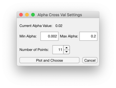
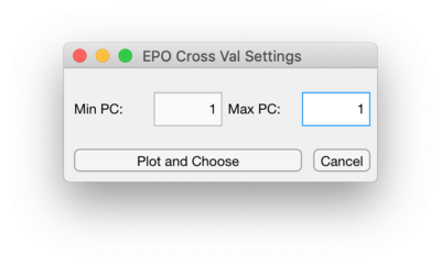
Opening the CV Window will allow setting a range alpha values to cross-validate over for GLSW or setting a range of number of PCs to cross-validate over for EPO. Use the Number of Points to set this range of alpha values. The alpha value range will be logarithmically spaced. To set the range of PCs to cross-validate over for EPO, change the Max PC value to be the desired maximum PC.
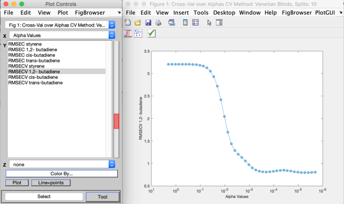
The Plot and Choose button in this window will plot the cross-validation results and will allow selecting the alpha value or PC to use for final model building. This will be a PlotGUI plot where the RMSEC and RMSECV results can be plotted via the Plot Controls window for the different properties of interest. The cross-validate method and parameters used is shown in the figure name at the very top of this figure window. Use the "Choose SINGLE value to keep" button, left most button, to select a single point to be your alpha or PC to use for final model building. Once a value is selected use the green check button to accept the selection and close this plot. Use the "Include All" button, the middle button, to reset the selection and choose a different value.


