Model Application: Validation Phase: Difference between revisions
imported>Jeremy No edit summary |
imported>Jeremy No edit summary |
||
| Line 6: | Line 6: | ||
Regardless of the analysis method, the Test and Validation phase consists of the same general series of steps: | Regardless of the analysis method, the Test and Validation phase consists of the same general series of steps: | ||
{| | {| | ||
|- | |- | ||
| Line 16: | Line 16: | ||
|} | |} | ||
{| | {| | ||
|- | |- | ||
| Line 26: | Line 26: | ||
|} | |} | ||
{| | {| | ||
|- | |- | ||
| Line 46: | Line 46: | ||
You have a variety of options for opening an Analysis window and loading data. Because these methods have been discussed in detail in other areas of the documentation, they are not repeated here. Instead, a brief summary is provided with a cross-reference to the detailed information. Simply choose the method that best fits your working needs. | You have a variety of options for opening an Analysis window and loading data. Because these methods have been discussed in detail in other areas of the documentation, they are not repeated here. Instead, a brief summary is provided with a cross-reference to the detailed information. Simply choose the method that best fits your working needs. | ||
{| | {| | ||
|- | |- | ||
| Line 55: | Line 55: | ||
|} | |} | ||
{| style="margin-left:18pt" | {| style="margin-left:18pt" | ||
|- | |- | ||
| Line 64: | Line 64: | ||
|} | |} | ||
{| style="margin-left:18pt" | {| style="margin-left:18pt" | ||
|- | |- | ||
| Line 73: | Line 73: | ||
|} | |} | ||
{| style="margin-left:18pt" | {| style="margin-left:18pt" | ||
|- | |- | ||
| Line 84: | Line 84: | ||
:Note: For information about working with icons in the Workspace Browser, see [[WorkspaceBrowser_DataIcons|Icons in the Workspace Browser]]. | :Note: For information about working with icons in the Workspace Browser, see [[WorkspaceBrowser_DataIcons|Icons in the Workspace Browser]]. | ||
{| | {| | ||
|- | |- | ||
| Line 93: | Line 93: | ||
|} | |} | ||
{| style="margin-left:18pt" | {| style="margin-left:18pt" | ||
|- | |- | ||
| Line 102: | Line 102: | ||
|} | |} | ||
{| style="margin-left:18pt" | {| style="margin-left:18pt" | ||
|- | |- | ||
| Line 111: | Line 111: | ||
|} | |} | ||
{| style="margin-left:18pt" | {| style="margin-left:18pt" | ||
|- | |- | ||
| Line 120: | Line 120: | ||
|} | |} | ||
{| style="margin-left:18pt" | {| style="margin-left:18pt" | ||
|- | |- | ||
| Line 143: | Line 143: | ||
After you have opened the Analysis window and loaded the validation data, you then apply the model to the validation data. To apply the model to the validation data, you can do one of the following: | After you have opened the Analysis window and loaded the validation data, you then apply the model to the validation data. To apply the model to the validation data, you can do one of the following: | ||
{| | {| | ||
|- | |- | ||
| Line 152: | Line 152: | ||
|} | |} | ||
{| | {| | ||
|- | |- | ||
| Line 182: | Line 182: | ||
Note: The examples listed here are not meant to be an exhaustive list of all of the available Plot Controls options for refining a model using a Scores plot. Instead, it is simply to provide representative examples of some of the more commonly used options when applying a model. | Note: The examples listed here are not meant to be an exhaustive list of all of the available Plot Controls options for refining a model using a Scores plot. Instead, it is simply to provide representative examples of some of the more commonly used options when applying a model. | ||
{| | {| | ||
|- | |- | ||
| Line 202: | Line 202: | ||
:: | :: | ||
{| | {| | ||
|- | |- | ||
| Line 212: | Line 212: | ||
|} | |} | ||
{| | {| | ||
|- | |- | ||
| Line 222: | Line 222: | ||
|} | |} | ||
{| style="margin-left:18pt" | {| style="margin-left:18pt" | ||
|- | |- | ||
| Line 233: | Line 233: | ||
Note: You should review a variety of plots with just the validation data, and then with both the validation data and calibration data to ensure that your validation data has the same distribution as your calibration data. For example, plot the Q Residuals versus the T^2 values for the validation data alone, then click the Show Cal Data with Test option to add the calibration data to this plot to confirm that your validation samples cover the same "space" (low Q/low T^2) that your calibration samples cover. | Note: You should review a variety of plots with just the validation data, and then with both the validation data and calibration data to ensure that your validation data has the same distribution as your calibration data. For example, plot the Q Residuals versus the T^2 values for the validation data alone, then click the Show Cal Data with Test option to add the calibration data to this plot to confirm that your validation samples cover the same "space" (low Q/low T^2) that your calibration samples cover. | ||
{| style="margin-left:18pt" | {| style="margin-left:18pt" | ||
|- | |- | ||
| Line 242: | Line 242: | ||
|} | |} | ||
{| style="margin-left:18pt" | {| style="margin-left:18pt" | ||
|- | |- | ||
| Line 251: | Line 251: | ||
|} | |} | ||
{| | {| | ||
|- | |- | ||
Revision as of 12:33, 29 July 2010
Table of Contents | Previous | Next
Applying the Model in the Test and Validation Phase
Regardless of the analysis method, the Test and Validation phase consists of the same general series of steps:
| 1. | Loading the validation data and applying the model to the validation data. See Loading the validation data and applying the model to the data. |
| 2. | Iteratively examining the model by focusing just on the validation data or on the validation data in the context of the calibration data and refining the model by adjusting the confidence limits and/or reducing the model complexity. See Examining and refining the model. |
| 3. | Saving the model. |
Note: Decomposition and Clustering analysis methods require only x block data to apply the model in the Test and Validation phase. Regression analysis methods require both x block data and y block data. Classification analysis methods require x block data with classes in either X or Y. For simplicity and brevity, this section describes model application during the Test and Validation phase using a simple PCA model; however, all of the general information in this section is applicable for all analysis methods.
Note: For a review of building this example PCA model during the Calibration phase, see Building the Model in the Calibration Phase.
Note: To review a detailed description of the Test and Validation phase, see Chapter 12, "Analysis Phases," on page 69.
Loading the validation data and applying the model to the data
You have a variety of options for opening an Analysis window and loading data. Because these methods have been discussed in detail in other areas of the documentation, they are not repeated here. Instead, a brief summary is provided with a cross-reference to the detailed information. Simply choose the method that best fits your working needs.
|
|
|
|
- Note: For information about working with icons in the Workspace Browser, see Icons in the Workspace Browser.
|
|
|
|
|
- Note: For information about the data manipulation options on the context menu, see Icons in the Workspace Browser or Importing Data into the Workspace Browser. For information about loading items from the Model Cache pane, see Analysis window Model Cache pane.
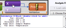
Also, remember that after you load data into a validation control, you can place your mouse pointer on the control to view not only information about the loaded data, but also, different instructions about working with the control. In the figure below, data has been loaded into the X validation control for a PCA analysis.
- Viewing information about loaded data
After you have opened the Analysis window and loaded the validation data, you then apply the model to the validation data. To apply the model to the validation data, you can do one of the following:
|
- Clicking the model control to apply the model to validation data
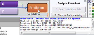
After the model is applied to the validation data, you can place your mouse pointer on the Model control to view information about the model.
- Viewing information about the model
Examining and refining the model
After the model is applied, the most relevant plots to create are Scores plots. (Remember, nothing has changed about the Eigenvalues, nothing has changed about the loads and variable statistics - all you have done is apply the model to validation data.)
Note: The examples listed here are not meant to be an exhaustive list of all of the available Plot Controls options for refining a model using a Scores plot. Instead, it is simply to provide representative examples of some of the more commonly used options when applying a model.
| 1. | On the Analysis window toolbar.click the Plot scores and sample statistics button |
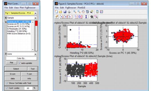
- The figure below shows some of the possible Scores plots for when applying the PCA model that you built during the Calibration phase to validation data. Note that initially, the plots show both the calibration data (
 ) and the validation data (
 ).
).
- Scores plot showing both calibration data and validation data
| 2. | Double-click on a plot of interest in the multiplot Figure window to open the plot in its own Figure window, or you can select the plot in the multiplot Figure window, and on the Plot Controls window, click View > Subplots. |
| 3. | With the plot of interest now open in its own Figure window, you can now do one or more of the following to refine the model: |
|
Note: You should review a variety of plots with just the validation data, and then with both the validation data and calibration data to ensure that your validation data has the same distribution as your calibration data. For example, plot the Q Residuals versus the T^2 values for the validation data alone, then click the Show Cal Data with Test option to add the calibration data to this plot to confirm that your validation samples cover the same "space" (low Q/low T^2) that your calibration samples cover.
|
|
| 4. | After you are satisfied with the model, save the model. |


