MIA Toolbox Texture Quick Start

Previous Topic: Loading Image Data

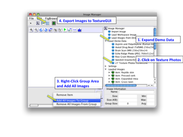
This example uses the textures demo dataset. Load textures by clicking on Load Demo Data in the tree, then 27 Texture Photos. This will load the data into Image Manager. Right-click in the image group area and select Add All Images to Group then click the Export to Texture button.

The Texture interface will open with textures loaded. Next, select Fourier Transform (fft) from the Texture Method drop-down menu and use the default Rows for the Spectrum Direction. Now click Calculate to create the spectra and display them.

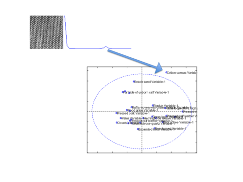
To get a better understanding of how the images are related, let's export the spectra to Analysis and create a PCA model. Here are the steps: In the Texture Interface, click the Export to Analysis button. When Analysis opens, select PCA from the Analysis menu. Click the model icon or calculate button (gears icon) to calculate a model (use the default number of PCs). Open a scores plot by clicking on the Plot Scores button. Double click the PC 1 vs PC 2 plot (upper right) to open it in a separate figure. Add labels using the Plot Controls View>Labels>Set One. You can see there's one real "oddball" in the PC 1 vs PC 2 plot, the Cotton Canvas. If you go back an look at the image you can see that it's highly "regular" in its texture and has a pronounced feature in its spectrum.

Next Topic: Review Results