Batchmaturity and Modeloptimizergui: Difference between pages
imported>Donal |
imported>Mathias |
||
| Line 1: | Line 1: | ||
== | =Model Optimizer= | ||
__TOC__ | |||
=Introduction= | |||
Optimizing modeling conditions and settings requires building and comparing multiple models. The Model Optimizer allows you to both automate building of models and visualize a comparison of models. See the [[modeloptimizer]] and [[comparemodels]] functions for more additional command line information. | |||
The interface is based around the idea of a "Snapshot" of the Analysis model building interface. Each snapshot contains all the settings for building the model. Once a set of snapshots has been created, the Model Optimizer can assemble all combinations of the settings into a collection of models to calculate. This collection can then be run at a convenient time or saved and run on new data. | |||
After all models have been calculated the results are displayed in a comparison table. By default the table shows only columns that differ between the models but it can be customized. Each column can be sorted to investigate results. | |||
'''Unsupported Model Types''' | |||
* CLUSTER | |||
* PURITY | |||
* Batch Maturity | |||
=Model Optimizer Interface= | |||
==Getting Started== | |||
Snapshots can be take from the Analysis toolbar or the Model Optimizer toolbar by clicking the snapshot button (camera icon). Each time a snapshot is taken the settings are added to the snapshot list as well as the model list. The combinations are updated after each snapshot. A Model Optimizer window will open if it's not already. | |||
Once you've added the desired snapshots you can either calculate the list of models immediately or click the '''Add Combinations''' button to add all unique combinations of the model settings to the models list then calculate. | |||
After the models are calculated the model comparison table will be updated showing the columns that differ between models. Sort the columns to find models with the desired value. For additional information on each model, expand it's leaf in the tree. | |||
==Taking Snapshots== | |||
A snapshot can be taken before or after a model is calculated (by clicking the Snapshot button). | |||
* If the snapshot is taken before calculation it will be added to both the Snapshot List and Model List but no results will be available until it's calculated. Any additional combinations resulting from the Snapshot will not be added to the Model List, you must add those by by clicking Add Combinations button. | |||
* If the snapshot is taken after calculation, the model will be added same as above but results will be displayed immediately in the Comparison Table. | |||
If you have large data and or time-consuming model settings it's often useful to take a Snapshot '''without''' calculating the model. Then, adjust settings and continue assembling snapshots '''without''' calculating. Once you have all the models assembled you can create them (all at once) from the Model Optimizer. | |||
Use Combinations to generate all unique combinations of model settings. For example, if you change the cross-validation and preprocessing, take a snapshot, then change cross-validation and preprocessing again and take a snapshot, there will be 4 possible combinations. Clicking the Add Combinations button will add all 4. | |||
== | ==Model Optimizer Window== | ||
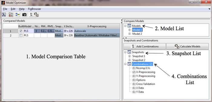
The main Optimizer Window has 4 sections: | |||
[[ | # Model comparison table. | ||
# Model list. | |||
# Snapshot list. | |||
# Combinations list. | |||
[[Image:ModelOptimizerMain.png|700px|GUI Window]] | |||
==Managing Snapshots and Models== | |||
Clicking the snapshot button adds it to the snapshot list, updates the combinations list, and adds the snapshot to the model list. A snapshot or model can be removed by clicking the '''Remove''' node in the list tree or by using the right-click menu. | |||
The list right-click menu allows you to: | |||
* Collapse all leafs in the tree. | |||
* Run all models. | |||
* Add a single snapshot to the model list. | |||
* Add all snapshots to model list. | |||
* Clear a single snapshot or model from the list. | |||
* Clear all snapshots or models from the list. | |||
* Clear everything. | |||
Expanding each node will "drill down" into the snapshot/model settings. Expand a node to get more information about the item. | |||
==Survey Preprocessing== | |||
Preprocessing in a snapshot can be "surveyed" over a range of parameter values via the [[preprocessiterator | preprocess iteration]] function. | |||
# Create a snapshot with the preprocessing you wish to survey. | |||
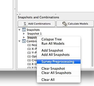
# Right-click on the snapshot and select "Survey Preprocessing" from the menu. | |||
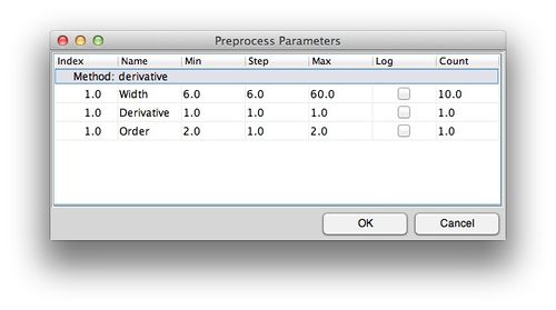
# For each of the preprocessing methods available for surveying (see [[preprocessiterator]] for a list) select the min, max and interval to use. '''Note:''' a full factorial of the combinations will be created so the total number of models will be the product of the "count" column. | |||
# Click '''OK''' and the new snapshots should appear. You can expand the snapshots to confirm preprocess settings. | |||
# Click '''Add Combinations''' then '''Calculate Models'''. | |||
<br> | |||
Survey Menu: | |||
[[Image:SurveyPreprocessingMenu.jpg||300px| ]] | |||
Survey Figure: | |||
[[Image:PreprocessIteratorFig.jpg| |500px| ]] | |||
==Adding Models from Cache or Workspace== | |||
Models can be added to the Optimizer from the cache or workspace by dragging and dropping them onto the window. If a model is added from the workspace the associated data is not added. | |||
A model can be added from the cache using the right-click menu "Compare" item. | |||
==Working with the Comparison Table== | |||
Once models have been added and calculated the Comparison Table will be updated. By default, only the columns with differing values will be displayed (columns with the same value for all models will be hidden). Investigate the results by sorting columns. | |||
The display of columns and table behavior can be modified via the Edit menu Include/Exclude Columns and the Options editor. Excluded columns do not appear in the include list so remove excluded columns from the exclude list before attempting to include them. | |||
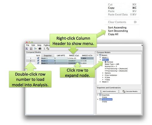
Right-click on the column header to display a context menu for sorting. Clicking on a particular row will expand the models corresponding node in the model tree. Double clicking the row number will open the model in analysis. | |||
[[Image:OptimizerTable.jpg| |500px|Optimizer Table]] | |||
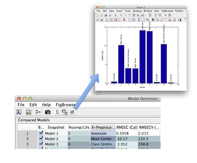
Click the plot button to generate a plot of the table data. | |||
[[Image:modeloptimizer_plot.jpg | |400px|Optimizer Plot]] | |||
==Saving an Optimizer Model== | |||
Optimizer models can be save from the '''File''' menu. These models are also "cached" in the model cache each time the '''Calculate''' button is pushed. | |||
=Applying New Data= | |||
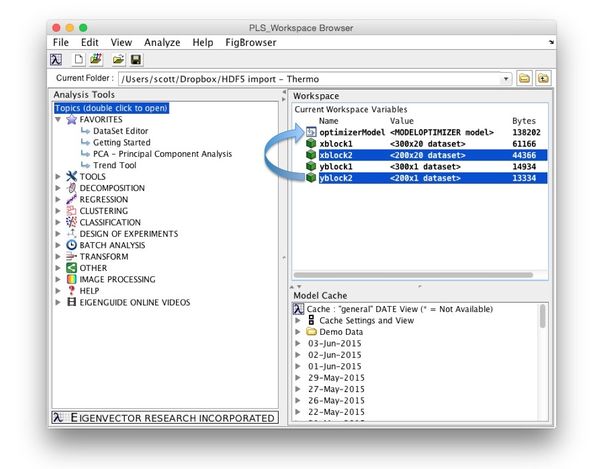
New data can be applied to an Optimizer model by dragging and dropping new data onto a model in the [[Workspace_Browser | Workspace Browser]]. | |||
* Locate the Model Optimizer model in the model cache and double-click it to load it into the workspace. | |||
* Load the data you want to apply. | |||
* Drag and drop new data onto your model. | |||
* Once the model is calculated you'll be prompted to save the model to the workspace. | |||
* Double-click the new model to open it in the Model Optimizer window. | |||
[[Image:ApplyModelOptimizer.jpg||600px|Apply Optimizer]] | |||
[[Image:modeloptimizer1.jpg||600px|Validate Optimizer]] | |||
=Applying Validation Data= | |||
[[Image:modeloptimizer1.jpg||600px|Validate Optimizer]] | |||
Revision as of 21:41, 17 October 2016
Model Optimizer
Introduction
Optimizing modeling conditions and settings requires building and comparing multiple models. The Model Optimizer allows you to both automate building of models and visualize a comparison of models. See the modeloptimizer and comparemodels functions for more additional command line information.
The interface is based around the idea of a "Snapshot" of the Analysis model building interface. Each snapshot contains all the settings for building the model. Once a set of snapshots has been created, the Model Optimizer can assemble all combinations of the settings into a collection of models to calculate. This collection can then be run at a convenient time or saved and run on new data.
After all models have been calculated the results are displayed in a comparison table. By default the table shows only columns that differ between the models but it can be customized. Each column can be sorted to investigate results.
Unsupported Model Types
- CLUSTER
- PURITY
- Batch Maturity
Model Optimizer Interface
Getting Started
Snapshots can be take from the Analysis toolbar or the Model Optimizer toolbar by clicking the snapshot button (camera icon). Each time a snapshot is taken the settings are added to the snapshot list as well as the model list. The combinations are updated after each snapshot. A Model Optimizer window will open if it's not already.
Once you've added the desired snapshots you can either calculate the list of models immediately or click the Add Combinations button to add all unique combinations of the model settings to the models list then calculate.
After the models are calculated the model comparison table will be updated showing the columns that differ between models. Sort the columns to find models with the desired value. For additional information on each model, expand it's leaf in the tree.
Taking Snapshots
A snapshot can be taken before or after a model is calculated (by clicking the Snapshot button).
- If the snapshot is taken before calculation it will be added to both the Snapshot List and Model List but no results will be available until it's calculated. Any additional combinations resulting from the Snapshot will not be added to the Model List, you must add those by by clicking Add Combinations button.
- If the snapshot is taken after calculation, the model will be added same as above but results will be displayed immediately in the Comparison Table.
If you have large data and or time-consuming model settings it's often useful to take a Snapshot without calculating the model. Then, adjust settings and continue assembling snapshots without calculating. Once you have all the models assembled you can create them (all at once) from the Model Optimizer.
Use Combinations to generate all unique combinations of model settings. For example, if you change the cross-validation and preprocessing, take a snapshot, then change cross-validation and preprocessing again and take a snapshot, there will be 4 possible combinations. Clicking the Add Combinations button will add all 4.
Model Optimizer Window
The main Optimizer Window has 4 sections:
- Model comparison table.
- Model list.
- Snapshot list.
- Combinations list.
Managing Snapshots and Models
Clicking the snapshot button adds it to the snapshot list, updates the combinations list, and adds the snapshot to the model list. A snapshot or model can be removed by clicking the Remove node in the list tree or by using the right-click menu.
The list right-click menu allows you to:
- Collapse all leafs in the tree.
- Run all models.
- Add a single snapshot to the model list.
- Add all snapshots to model list.
- Clear a single snapshot or model from the list.
- Clear all snapshots or models from the list.
- Clear everything.
Expanding each node will "drill down" into the snapshot/model settings. Expand a node to get more information about the item.
Survey Preprocessing
Preprocessing in a snapshot can be "surveyed" over a range of parameter values via the preprocess iteration function.
- Create a snapshot with the preprocessing you wish to survey.
- Right-click on the snapshot and select "Survey Preprocessing" from the menu.
- For each of the preprocessing methods available for surveying (see preprocessiterator for a list) select the min, max and interval to use. Note: a full factorial of the combinations will be created so the total number of models will be the product of the "count" column.
- Click OK and the new snapshots should appear. You can expand the snapshots to confirm preprocess settings.
- Click Add Combinations then Calculate Models.
Survey Menu:
Survey Figure:
Adding Models from Cache or Workspace
Models can be added to the Optimizer from the cache or workspace by dragging and dropping them onto the window. If a model is added from the workspace the associated data is not added.
A model can be added from the cache using the right-click menu "Compare" item.
Working with the Comparison Table
Once models have been added and calculated the Comparison Table will be updated. By default, only the columns with differing values will be displayed (columns with the same value for all models will be hidden). Investigate the results by sorting columns.
The display of columns and table behavior can be modified via the Edit menu Include/Exclude Columns and the Options editor. Excluded columns do not appear in the include list so remove excluded columns from the exclude list before attempting to include them.
Right-click on the column header to display a context menu for sorting. Clicking on a particular row will expand the models corresponding node in the model tree. Double clicking the row number will open the model in analysis.
Click the plot button to generate a plot of the table data.
Saving an Optimizer Model
Optimizer models can be save from the File menu. These models are also "cached" in the model cache each time the Calculate button is pushed.
Applying New Data
New data can be applied to an Optimizer model by dragging and dropping new data onto a model in the Workspace Browser.
- Locate the Model Optimizer model in the model cache and double-click it to load it into the workspace.
- Load the data you want to apply.
- Drag and drop new data onto your model.
- Once the model is calculated you'll be prompted to save the model to the workspace.
- Double-click the new model to open it in the Model Optimizer window.
