Maf and MIA Toolbox PCA Quick Start: Difference between pages
imported>Scott No edit summary |
imported>Scott No edit summary |
||
| Line 1: | Line 1: | ||
=== | [[Loading Data Quick Start | Previous Topic: Loading Data]] | ||
{| border="1" cellpadding="5" cellspacing="0" align="left" | |||
= | |- | ||
: | |valign="top" | | ||
[[Image:LoadExportSMBread.png |right |(Click to Enlarge)]] | |||
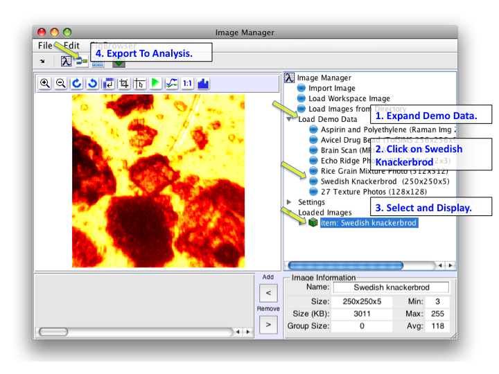
This example uses the '''smbread''' dataset. Load '''smbread''' by clicking on '''Load Demo Data''' in the tree, then '''Swedish Knackerbrod'''. This will load the data into Image Manager. Click on the item in the Loaded Images section to view it and make it the current selected image. Next, click on the export to Analysis button. This will open the Analysis GUI and load '''smbread'''. | |||
|- | |||
|valign="top" | | |||
[[Image:RecalcBreadImage4PCs.png |right| 500px |(Click to Enlarge)]] | |||
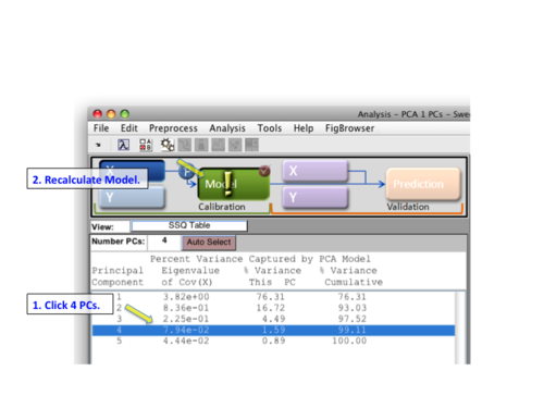
The Analysis interface will open with '''smbread''' loaded. Next, select '''PCA''' from the '''Analysis''' menu and then click the '''Model''' icon in the Status Pane. By default a model with one PC will be calculated. Let's try 4 PCs by selecting row 4 and clicking the '''Model''' icon again. | |||
|- | |||
|valign="top"| | |||
[[Image:build_model.004.png |right| 500px |(Click to Enlarge)]] | |||
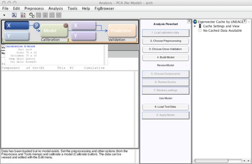
The Analysis GUI will then appear with the given data already loaded. (The large '''X''' (block) button in the Analysis GUI will appear depressed indicating the data is loaded - passing the cursor over the button will provide a summary of the '''X''' block data.) | |||
|- | |||
|valign="top"| | |||
[[Image:build_model.005.png |right| 500px |(Click to Enlarge)]] | |||
While each analysis type has its own nuances, in general the steps to build a model are: | |||
# load the data | |||
# view the data | |||
# choose preprocessing | |||
# select the type of cross-validation to use (if any is desired - see [[Using Cross-Validation]]) | |||
# build the model | |||
# review the model | |||
[[ | |||
There is more than one way to accomplish each of the above steps. For example, preprocessing can be set for the '''X''' block by | |||
* clicking the '''"Choose Preprocessing"''' button in the Analysis Flowchart | |||
* clicking the '''P''' button next to the '''X''' button | |||
* select '''"Preprocess"''' menu item | |||
('''Hint:''' Once selected, use the Preprocess/X-block and Preprocess/Y-block menus to save the current preprocessing as the default.) | |||
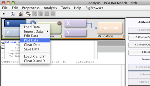
You can quickly view your data by right-clicking on the appropriate button ('''X''' or '''Y''') and then select '''"Plot Data"''' | |||
|- | |||
|valign="top"| | |||
[[Image:build_model.006.png|right| |(Click to Enlarge)]] | |||
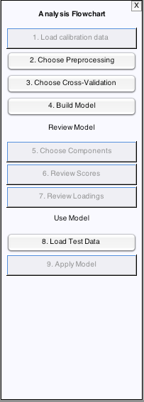
Perhaps the quickest way for new users to complete the remaining steps to build the model is to use the flowchart. | |||
|} | |||
[[Review Results Quick Start | Next Topic: Review Results]] | |||
Revision as of 17:41, 9 October 2009
|
This example uses the smbread dataset. Load smbread by clicking on Load Demo Data in the tree, then Swedish Knackerbrod. This will load the data into Image Manager. Click on the item in the Loaded Images section to view it and make it the current selected image. Next, click on the export to Analysis button. This will open the Analysis GUI and load smbread. |
|
The Analysis interface will open with smbread loaded. Next, select PCA from the Analysis menu and then click the Model icon in the Status Pane. By default a model with one PC will be calculated. Let's try 4 PCs by selecting row 4 and clicking the Model icon again. |
|
The Analysis GUI will then appear with the given data already loaded. (The large X (block) button in the Analysis GUI will appear depressed indicating the data is loaded - passing the cursor over the button will provide a summary of the X block data.) |
|
While each analysis type has its own nuances, in general the steps to build a model are:
There is more than one way to accomplish each of the above steps. For example, preprocessing can be set for the X block by
(Hint: Once selected, use the Preprocess/X-block and Preprocess/Y-block menus to save the current preprocessing as the default.) You can quickly view your data by right-clicking on the appropriate button (X or Y) and then select "Plot Data" |
|
Perhaps the quickest way for new users to complete the remaining steps to build the model is to use the flowchart. |
